Introduction:
In this experiment, we will realize K-means clustering algorithm (K-means) and understand its working principle in data clustering and its application in image compression.
The data sets used in this experiment include:
- ex3data1.mat -2D dataset
- hzau.jpeg - an image used to test the image compression performance of k-means clustering algorithm
The scoring criteria are as follows:
- Point 1: find the nearest class center -----------------(20 points)
- Point 2: calculate the mean class center --------------------(20 points)
- Point 3: randomly initialize the class center -----------------(10 points)
- Key point 4: K-means clustering algorithm ---------------------(20 points)
- Point 5: image compression -----------------------------(30 points)
In [1]:
# Import the required library files
import os
import numpy as np
import pandas as pd
import matplotlib.pyplot as plt
import matplotlib as mpl
import seaborn as sb
from scipy.io import loadmat

%matplotlib inline
1 K-means Clustering
In this part of the experiment, the K-means clustering algorithm will be implemented.
In each iteration, the algorithm mainly includes two parts: finding the nearest class center and calculating the mean class center.
In addition, based on the needs of initialization, it is necessary to create a function to select random samples and use them as the initial cluster center.
1.1 find the nearest Center
In this part of the experiment, we will find the nearest class center for each sample point and assign it to the corresponding class.
The specific update formula is as follows:
ci:=argminj=1,⋯,K∥xi−μj∥2,ci:=argminj=1,⋯,K‖xi−μj‖2,
Where xixi is the second sample point, μ j μ J is the center of the jj mean class.
**Important point 1: * * in the cell below, please * * implement the code of "finding the nearest class center" * *.
In [2]:
# ======================Fill in the code here=======================
def find_closest_centroids(X, centroids):
    """
    input
    ----------
    X : Size (m, n)Matrix of, page i Act No i Samples, n Is the dimension of the sample.

    centroids : Size (k, n)Matrix of, where k Is the number of categories.

    output
    -------
    idx : Size (m, 1)Matrix of, page i The first component represents the second component i Category of samples.
    """
    m = X.shape[0]
    k = centroids.shape[0]
    idx = np.zeros(m,dtype=np.int)

    for i in range(m):
        minn = 100000
        for j in range(k):
            dist = np.sum((X[i,:] - centroids[j,:]) ** 2)
            if dist < minn:
                minn = dist
                idx[i] = j

    return idx
# =============================================================
If the above function is completed find_closest_centroids, the following code can be used for testing. If the result is [0 2 1], the calculation passes.
In [3]:
#Import data
data = loadmat('ex3data1.mat')
X = data['X']
X1=X
initial_centroids = np.array([[3, 3], [6, 2], [8, 5]])

idx = find_closest_centroids(X, initial_centroids)
idx[0:3]
Out[3]:
array([0, 2, 1])
In [4]:
#Display and view some data
data2 = pd.DataFrame(data.get('X'), columns=['X1', 'X2'])
data2.head()
Out[4]:
| X1 | X2 | |
|---|---|---|
| 0 | 1.842080 | 4.607572 |
| 1 | 5.658583 | 4.799964 |
| 2 | 6.352579 | 3.290854 |
| 3 | 2.904017 | 4.612204 |
| 4 | 3.231979 | 4.939894 |
In [5]:
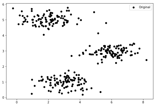
#Visualization of 2D data
fig, ax = plt.subplots(figsize=(9,6))
ax.scatter(X[:,0], X[:,1], s=30, color='k', label='Original')
ax.legend()
plt.show()

1.2 calculation of mean class center
In this part of the experiment, we take the mean of each class of samples as the new class center.
The specific update formula is as follows:
μj:=1|Cj|∑i∈Cjxiμj:=1|Cj|∑i∈Cjxi
Where cjcjj is the index set of the jj sample point and | CJ | CJ | is the number of elements of the set CjCj.
**Important point 2: * * in the cell below, please * * implement the code of "calculate mean class center" * *.
In [6]:
# ======================Fill in the code here=======================
def compute_centroids(X, idx, k):
    m, n = X.shape
    centroids = np.zeros((k, n))
    #print(n)
    for i in range(k):
        num=0
        sum=np.zeros(n)
        for j in range(m):
            if idx[j]==i:
                num=num+1
                sum[:]=sum[:]+X[j,:]
        centroids[i]=sum[:]/num


    return centroids
# =============================================================
In [7]:
#Test the above calculated mean class center code
compute_centroids(X, idx, 3)
Out[7]:
array([[2.42830111, 3.15792418],
       [5.81350331, 2.63365645],
       [7.11938687, 3.6166844 ]])
1.3 random initialization class center
k samples are randomly selected as the initial class center.
**Important 3: * * in the cell below, please * * implement the code of "random initialization class center" * *. Specifically, k samples are randomly selected as the initial class center.
In [8]:
# ======================Fill in the code here=======================
def init_centroids(X, k):
    m, n = X.shape
    #j=m/k
    #print(j)
    idx = np.random.randint(0, m, k)
    centroids = np.zeros((k, n))
    for i in range(k):
        centroids[i,:] = X[idx[i],:]

    return centroids
# =============================================================
In [9]:
#Test the above random initialization class center code
init_centroids(X, 3)
Out[9]:
array([[3.30063655, 1.28107588],
       [1.02285128, 5.0105065 ],
       [6.59702155, 3.07082376]])
1.4 realize K-means clustering algorithm
**Key point 4: * * in the cell below, please * * implement the code of "K-means clustering algorithm" by combining the above steps * *.
In [10]:
# ======================Fill in the code here=======================
def run_k_means(X, initial_centroids, max_iters):
    m, n = X.shape
    k = initial_centroids.shape[0]
    idx = np.zeros(m)
    #centroids = np.zeros((k, n))
    centroids =initial_centroids
    centroids_last =initial_centroids
    for i in range(max_iters):
        idx = find_closest_centroids(X, centroids)
        centroids = compute_centroids(X, idx, k)
        if (centroids==centroids_last).all()==True:
            break
        centroids_last = compute_centroids(X, idx, k)

    return idx, centroids
# =============================================================
2 apply K-means clustering algorithm to data set 1
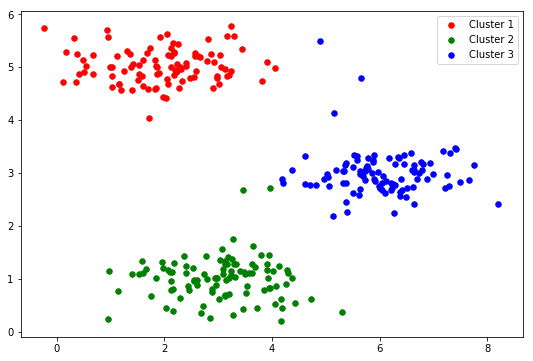
In this part of the experiment, the implemented K-means clustering algorithm is applied to data set 1. The sample dimension of the data set is 2. Therefore, after clustering, the clustering results can be observed visually.
In [11]:
idx, centroids = run_k_means(X, initial_centroids, 10)
# print(centroids)
In [12]:
cluster1 = X[np.where(idx == 0)[0],:]
cluster2 = X[np.where(idx == 1)[0],:]
cluster3 = X[np.where(idx == 2)[0],:]

fig, ax = plt.subplots(figsize=(9,6))
ax.scatter(cluster1[:,0], cluster1[:,1], s=30, color='r', label='Cluster 1')
ax.scatter(cluster2[:,0], cluster2[:,1], s=30, color='g', label='Cluster 2')
ax.scatter(cluster3[:,0], cluster3[:,1], s=30, color='b', label='Cluster 3')
ax.legend()
plt.show()

1.3 applying K-means clustering algorithm to image compression Image compression with K-means
In [13]:
#Read image
A = mpl.image.imread('hzau.jpeg')
A.shape
Out[13]:
(96, 150, 3)
Now we need to apply some preprocessing to the data and provide it to the K-means algorithm.
In [14]:
# Normalize the range of image pixel values to [0, 1]
A = A / 255.

# Transform the original image size
X = np.reshape(A, (A.shape[0] * A.shape[1], A.shape[2]))
X.shape
Out[14]:
(14400, 3)
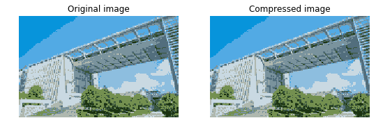
**Key point 5: * * in the cell below, * * Please use K-means clustering algorithm to realize image compression * *. The specific method is to replace the original pixel with the corresponding mean class center pixel.
In [21]:
# ======================Fill in the code here=======================
# Random initialization class center
initial_centroids = init_centroids(X, 16)
m=X.shape[0]
idx, centroids = run_k_means(X, initial_centroids, 10)
idx = find_closest_centroids(X, centroids)
#n=centroids.shape[0]
#print(n)
A_compressed=X
for i in range(m):
    A_compressed[i,:]=centroids[idx[i],:]
A_compressed = np.reshape(A_compressed, (96, 150,3))
print(A_compressed.shape)
# =============================================================
/opt/conda/lib/python3.6/site-packages/ipykernel_launcher.py:13: RuntimeWarning: invalid value encountered in true_divide del sys.path[0]
(96, 150, 3)
In [22]:
#Display images before and after compression
fig, ax = plt.subplots(1, 2, figsize=(9,6))
ax[0].imshow(A)
ax[0].set_axis_off()
ax[0].set_title('Original image')
ax[1].imshow(A_compressed)
ax[1].set_axis_off()
ax[1].set_title('Compressed image')
plt.show()
In [27]:
#Calculation class center point
# ======================Fill in the code here=======================
def Manhattan(x, y):
    # Defines the calculation of Manhattan distance
    return np.sum(np.abs(x-y))

def compute_mid(X, idx, k):
    m, n = X.shape
    centroids = np.zeros((k, n))
    for i in range(k):
        minn=10000
        for j in range(m):

            if idx[j]==i:
                sum=0

                for h in range(m):
                    if idx[h]==i and j!=h:
                        sum=sum+Manhattan(X[j,:],X[h,:])
                if sum<minn:
                    minn=sum
                    centroids[i,:] =X[j,:]
#     print(centroids)
    return centroids
In [28]:
#Implement k-center clustering algorithm
def run_k_mid(X, initial_centroids, max_iters):
    m, n = X.shape
    k = initial_centroids.shape[0]
    idx = np.zeros(m)

    centroids =initial_centroids
    centroids_last =initial_centroids
    for i in range(max_iters):
        idx = find_closest_centroids(X, centroids)
#         print(i)
#         print(idx)
        centroids = compute_mid(X, idx, k)
#         print(centroids)
        if (centroids==centroids_last).all()==True:
            break
        centroids_last = compute_mid(X, idx, k)

    return idx, centroids

# =============================================================
In [29]:
initial_centroids=init_centroids(X1, 3)
# print(initial_centroids)
idx, centroids = run_k_mid(X1, initial_centroids, 10)
# print(idx)
# print(centroids)
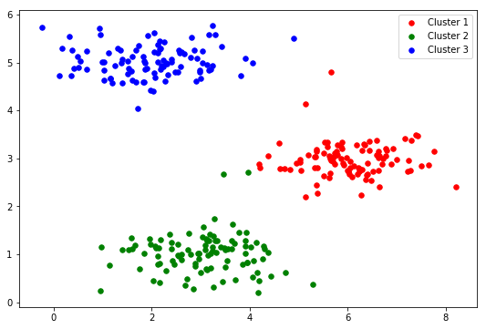
In [30]:
cluster1 = X1[np.where(idx == 0)[0],:]
cluster2 = X1[np.where(idx == 1)[0],:]
cluster3 = X1[np.where(idx == 2)[0],:]

fig, ax = plt.subplots(figsize=(9,6))
ax.scatter(cluster1[:,0], cluster1[:,1], s=30, color='r', label='Cluster 1')
ax.scatter(cluster2[:,0], cluster2[:,1], s=30, color='g', label='Cluster 2')
ax.scatter(cluster3[:,0], cluster3[:,1], s=30, color='b', label='Cluster 3')
ax.legend()
plt.show()
initial_centroids=init_centroids(X1, 3)
# print(initial_centroids)
idx, centroids = run_k_mid(X1, initial_centroids, 10)
# print(idx)
# print(centroids)
