(1) Background: forest fire refers to the behavior of forest fire that is out of human control, spreads and expands freely in the forest land, and brings certain harm and loss to the forest, forest ecosystem and human beings. Forest fire is a natural fire with strong sudden, destructive and difficult disposal and rescue. In recent years, due to the intensification of the greenhouse effect, forest fires occur frequently. In this way In the situation of, it is necessary to do a good job in prevention. To achieve 24-hour, all-weather and large-scale monitoring, satellite and UAV patrol are better measures. For UAV patrol, how machines judge the occurrence of fire in the current area, computer vision should be one of the important technologies, so a small program for forest fire picture recognition is designed, I hope to understand computer vision through this design.
(2) Machine learning design case design scheme: download relevant data sets from the website, sort out the data sets, label the files in the data set in the python environment, preprocess the data, use keras to build the network, train the model, and import the picture test model
Reference source: kaggle discussion area on label learning
Data set source: kaggle, website: https://www.kaggle.com/
(3) Implementation steps of machine learning:
1, Second classification
1. Download data set

2. Import the required library
 1 #Import required libraries
 2 import numpy as np
 3 import pandas as pd
 4 import os
 5 import tensorflow as tf
 6 import matplotlib.pyplot as plt
 7 from pathlib import Path
 8 from sklearn.model_selection import train_test_split
 9 from keras.models import Sequential
10 from keras.layers import Activation
11 from keras.layers import Dense, Dropout, Flatten, Conv2D, MaxPooling2D
12 from keras.applications.resnet import preprocess_input
13 from keras_preprocessing.image import ImageDataGenerator
14 from keras.models import load_model
15 from keras.preprocessing.image import load_img, img_to_array
16 from keras import optimizers
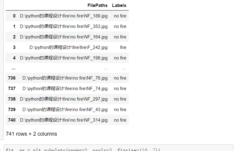
3. Traverse the files in the dataset and generate DataFrame from path data and label data
 1 dir = Path('D:/python Curriculum design 1/fire')
 2
 3 # use glob Traversal in dir All in path jpg Format and add all file names to the filepaths In the list
 4 filepaths = list(dir.glob(r'**/*.jpg'))
 5
 6 # Separate the divided small file name (category name) in the file and add it to the labels In the list of
 7 labels = list(map(lambda l: os.path.split(os.path.split(l)[0])[1], filepaths))
 8
 9 # take filepaths adopt pandas Convert to Series data type
10 filepaths = pd.Series(filepaths, name='FilePaths').astype(str)
11
12 # take labels adopt pandas Convert to Series data type
13 labels = pd.Series(labels, name='Labels').astype(str)
14
15 # take filepaths and Series Two Series Data type composition for DataFrame data type
16 df = pd.merge(filepaths, labels, right_index=True, left_index=True)
17 df = df[df['Labels'].apply(lambda l: l[-2:] != 'GT')]
18 df = df.sample(frac=1).reset_index(drop=True)
19 #View formed DataFrame Data
20 df
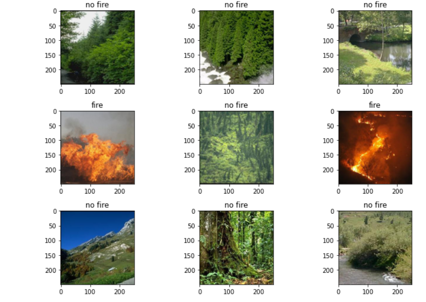
4. View the image and the corresponding label
 1 #View the image and the corresponding label
 2 fit, ax = plt.subplots(nrows=3, ncols=3, figsize=(10, 7))
 3
 4 for i, a in enumerate(ax.flat):
 5     a.imshow(plt.imread(df.FilePaths[i]))
 6     a.set_title(df.Labels[i])
 7
 8 plt.tight_layout()
 9 plt.show()
10
11 #View the number of pictures of each label
12 df['Labels'].value_counts(ascending=True)
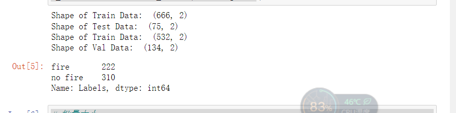
5. The training set, test set and verification set are generated from the total data set
 1 #The total data is distributed to the users in a ratio of 10:1 X_train, X_test
 2 X_train, X_test = train_test_split(df, test_size=0.1, stratify=df['Labels'])
 3
 4 print('Shape of Train Data: ', X_train.shape)
 5 print('Shape of Test Data: ', X_test.shape)
 6
 7 # Press 5 for the total data:1 Proportion allocated to X_train, X_train
 8 X_train, X_val = train_test_split(X_train, test_size=0.2, stratify=X_train['Labels'])
 9
10 print('Shape of Train Data: ', X_train.shape)
11 print('Shape of Val Data: ', X_val.shape)
12
13 # View the number of pictures of each label
14 X_train['Labels'].value_counts(ascending=True)
6. Image preprocessing
 1 # Batch size
 2 BATCH_SIZE = 32
 3 # Enter the size of the picture
 4 IMG_SIZE = (224, 224)
 5
 6 # Image preprocessing
 7 img_data_gen = ImageDataGenerator(preprocessing_function=preprocess_input)
 8
 9 X_train = img_data_gen.flow_from_dataframe(dataframe=X_train,
10                                           x_col='FilePaths',
11                                           y_col='Labels',
12                                           target_size=IMG_SIZE,
13                                           color_mode='rgb',
14                                           class_mode='binary',
15                                           batch_size=BATCH_SIZE,
16                                           seed=42)
17
18 X_val = img_data_gen.flow_from_dataframe(dataframe=X_val,
19                                           x_col='FilePaths',
20                                           y_col='Labels',
21                                           target_size=IMG_SIZE,
22                                           color_mode='rgb',
23                                           class_mode='binary',
24                                           batch_size=BATCH_SIZE,
25                                           seed=42)
26 X_test = img_data_gen.flow_from_dataframe(dataframe=X_test,
27                                           x_col='FilePaths',
28                                           y_col='Labels',
29                                           target_size=IMG_SIZE,
30                                           color_mode='rgb',
31                                           class_mode='binary',
32                                           batch_size=BATCH_SIZE,
33                                           seed=42)

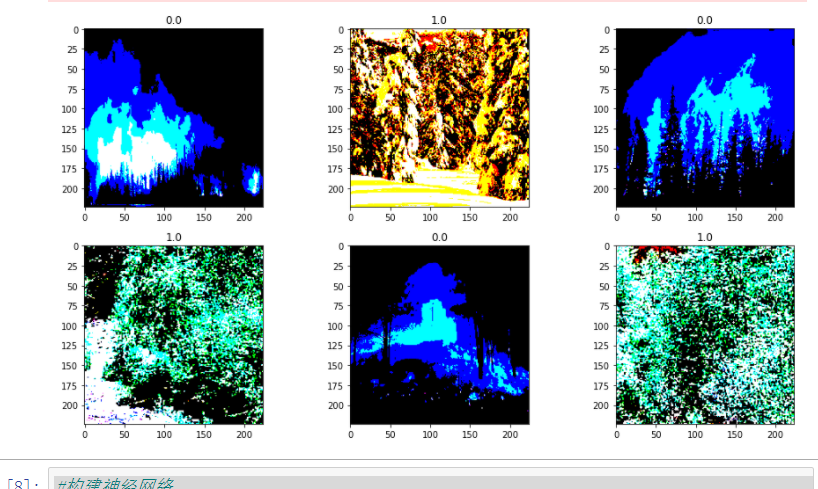
7. View the processed image and its binary tag
#View the processed picture and its binary label
fit, ax = plt.subplots(nrows=2, ncols=3, figsize=(13,7))

for i, a in enumerate(ax.flat):
    img, label = X_train.next()
    a.imshow(img[0],)
    a.set_title(label[0])

plt.tight_layout()
plt.show()
8. The neural network is constructed and the model is trained
#Constructing neural network
model = Sequential()
# Data normalization processing
model.add(tf.keras.layers.experimental.preprocessing.Rescaling(1./255))

# 1.Conv2D Layer, 32 filters
model.add(Conv2D(filters=32, kernel_size=(3,3), padding='same', input_shape=(224, 224, 3)))#The graphics are color,'rgb',So set 3
model.add(Activation('relu'))
model.add(MaxPooling2D(pool_size=(2,2), strides=2, padding='valid'))

# 2.Conv2D Layer, 64 filters
model.add(Conv2D(filters=64, kernel_size=(3,3), padding='same'))
model.add(Activation('relu'))
model.add(MaxPooling2D(pool_size=(2,2), strides=2, padding='valid'))

# 3.Conv2D Layer, 128 filters
model.add(Conv2D(filters=128, kernel_size=(3,3), padding='same'))
model.add(Activation('relu'))
model.add(MaxPooling2D(pool_size=(2,2), strides=2, padding='valid'))

# The data of the input layer is compressed into one-dimensional data, and the full connection layer can only process one-dimensional data
model.add(Flatten())

# Full connection layer
model.add(Dense(256))
model.add(Activation('relu'))

# Reduce overfitting
model.add(Dropout(0.5))

# Full connection layer
model.add(Dense(1))
model.add(Activation('sigmoid'))

# Model compilation
model.compile(optimizer=optimizers.RMSprop(lr=1e-4),
              loss="categorical_crossentropy",
              metrics=["accuracy"])
#Training model using batch generator
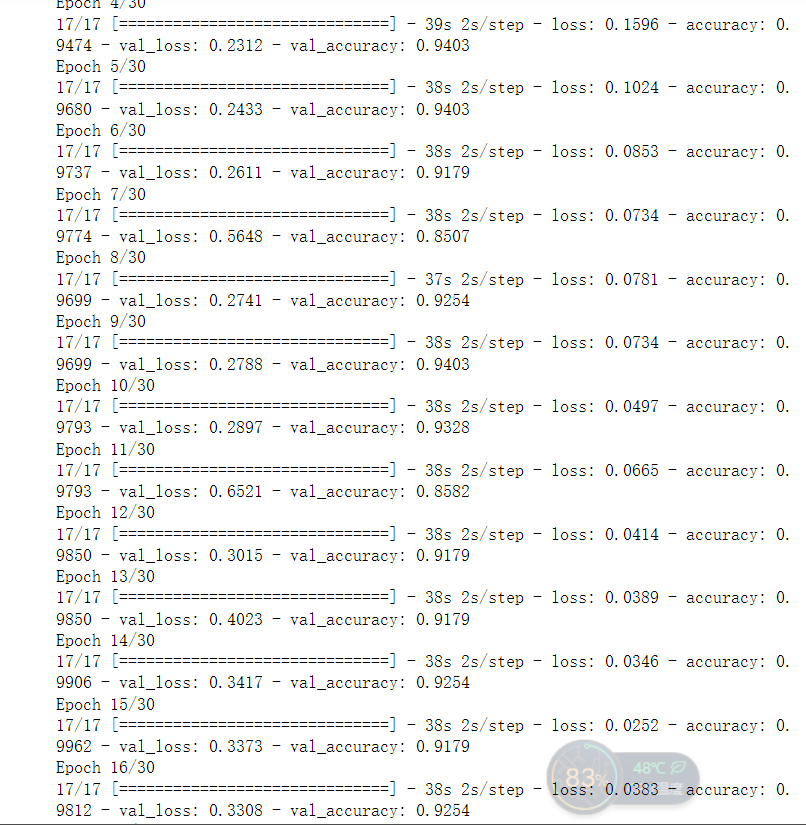
h1 = model.fit(X_train, validation_data=X_val,
epochs=30, )
#Save model
model.save('t1')
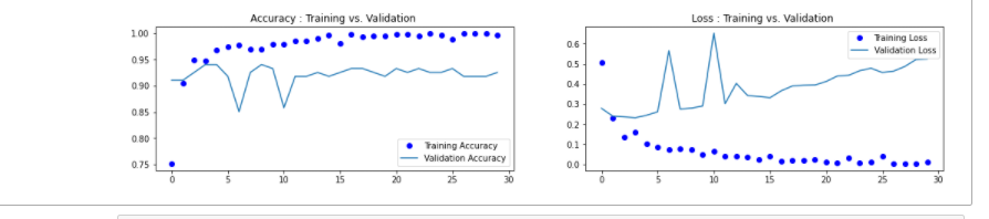
9. Draw loss curve and accuracy curve
 1 accuracy = h1.history['accuracy']
 2 loss = h1.history['loss']
 3 val_loss = h1.history['val_loss']
 4 val_accuracy = h1.history['val_accuracy']
 5 plt.figure(figsize=(17, 7))
 6 plt.subplot(2, 2, 1)
 7 plt.plot(range(30), accuracy,'bo', label='Training Accuracy')
 8 plt.plot(range(30), val_accuracy, label='Validation Accuracy')
 9 plt.legend(loc='lower right')
10 plt.title('Accuracy : Training vs. Validation ')
11 plt.subplot(2, 2, 2)
12 plt.plot(range(30), loss,'bo' ,label='Training Loss')
13 plt.plot(range(30), val_loss, label='Validation Loss')
14 plt.title('Loss : Training vs. Validation ')
15 plt.legend(loc='upper right')
16 plt.show()
10. Import pictures for prediction
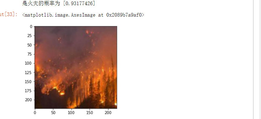
from PIL import Image
def con(file,outdir,w=224,h=224):
    img1=Image.open(file)
    img2=img1.resize((w,h),Image.BILINEAR)
    img2.save(os.path.join(outdir,os.path.basename(file)))
file='D:/python Curriculum design of/NA_Fish_Dataset/Black Sea Sprat/F_23.jpg'
con(file,'D:/python Curriculum design of/NA_Fish_Dataset/Black Sea Sprat/')
model=load_model('t1')
img_path='D:/python Curriculum design of/NA_Fish_Dataset/Black Sea Sprat/F_23.jpg'
img = load_img(img_path)
img = img_to_array(img)
img = np.expand_dims(img, axis=0)
out = model.predict(img)
if out[0]>0.5:
        print('The probability of fire is',out[0])
else:
         print('Not a fire')
img=plt.imread('D:/python Curriculum design of/NA_Fish_Dataset/Black Sea Sprat/F_23.jpg')
plt.imshow(img)
II. Multi classification
1. Prepare data set

2. Traverse the files in the dataset and generate DataFrame from path data and label data
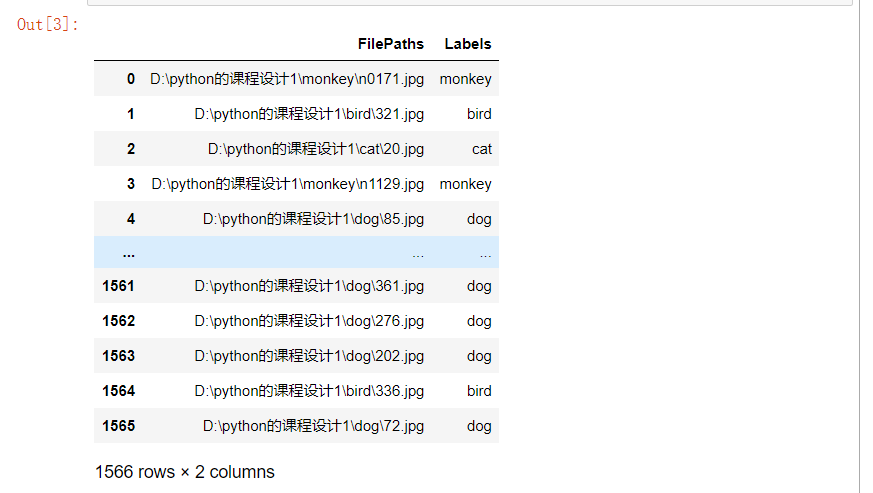
 1 dir = Path('D:/python Curriculum design 1')
 2
 3 # use glob Traversal in dir All in path jpg Format and add all file names to the filepaths In the list
 4 filepaths = list(dir.glob(r'**/*.jpg'))
 5
 6 # Separate the divided small file name (category name) in the file and add it to the labels In the list of
 7 labels = list(map(lambda l: os.path.split(os.path.split(l)[0])[1], filepaths))
 8
 9 # take filepaths adopt pandas Convert to Series data type
10 filepaths = pd.Series(filepaths, name='FilePaths').astype(str)
11
12 # take labels adopt pandas Convert to Series data type
13 labels = pd.Series(labels, name='Labels').astype(str)
14
15 # take filepaths and Series Two Series Data type composition for DataFrame data type
16 df = pd.merge(filepaths, labels, right_index=True, left_index=True)
17 df = df[df['Labels'].apply(lambda l: l[-2:] != 'GT')]
18 df = df.sample(frac=1).reset_index(drop=True)
#View the data of the formed DataFrame
df
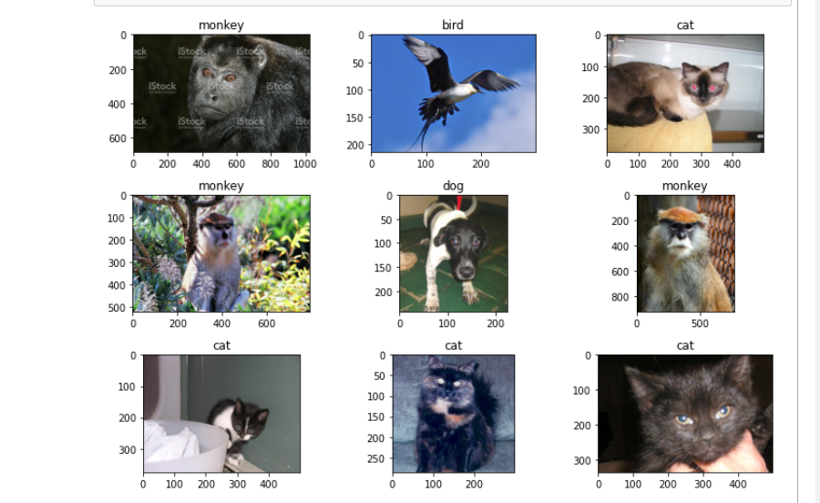
3. View the image and the corresponding label
1 fit, ax = plt.subplots(nrows=3, ncols=3, figsize=(10, 7))
2
3 for i, a in enumerate(ax.flat):
4     a.imshow(plt.imread(df.FilePaths[i]))
5     a.set_title(df.Labels[i])
6
7 plt.tight_layout()
8 plt.show()
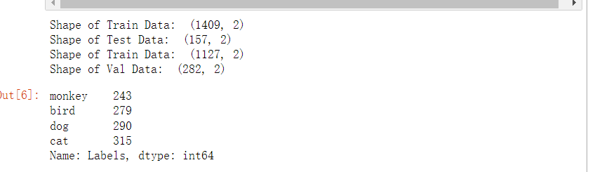
4. The training set, test set and verification set are generated from the total data set
#The total data is distributed to the users in a ratio of 10:1 X_train, X_test
X_train, X_test = train_test_split(df, test_size=0.1, stratify=df['Labels'])

print('Shape of Train Data: ', X_train.shape)
print('Shape of Test Data: ', X_test.shape)

# Press 5 for the total data:1 Proportion allocated to X_train, X_train
X_train, X_val = train_test_split(X_train, test_size=0.2, stratify=X_train['Labels'])

print('Shape of Train Data: ', X_train.shape)
print('Shape of Val Data: ', X_val.shape)

# View the number of pictures of each label
X_train['Labels'].value_counts(ascending=True)
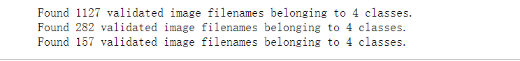
5. Image preprocessing
 1 # Batch size
 2 BATCH_SIZE = 32
 3 # Enter the size of the picture
 4 IMG_SIZE = (224, 224)
 5
 6 # Image preprocessing
 7 img_data_gen = ImageDataGenerator(preprocessing_function=preprocess_input)
 8
 9
10 X_train = img_data_gen.flow_from_dataframe(dataframe=X_train,
11                                           x_col='FilePaths',
12                                           y_col='Labels',
13                                           target_size=IMG_SIZE,
14                                           color_mode='rgb',
15                                           class_mode='categorical',
16                                           batch_size=BATCH_SIZE,
17                                           seed=42)
18
19 X_val = img_data_gen.flow_from_dataframe(dataframe=X_val,
20                                           x_col='FilePaths',
21                                           y_col='Labels',
22                                           target_size=IMG_SIZE,
23                                           color_mode='rgb',
24                                           class_mode='categorical',
25                                           batch_size=BATCH_SIZE,
26                                           seed=42)
27 X_test = img_data_gen.flow_from_dataframe(dataframe=X_test,
28                                           x_col='FilePaths',
29                                           y_col='Labels',
30                                           target_size=IMG_SIZE,
31                                           color_mode='rgb',
32                                           class_mode='categorical',
33                                           batch_size=BATCH_SIZE,
34                                           seed=42)
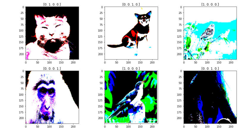
6. View the processed image and its one hot tag
1 fit, ax = plt.subplots(nrows=2, ncols=3, figsize=(13,7))
2
3 for i, a in enumerate(ax.flat):
4     img, label = X_train.next()
5     a.imshow(img[0],)
6     a.set_title(label[0])
7
8 plt.tight_layout()
9 plt.show()
7. Constructing neural network and training model
 1 model = Sequential()
 2 # Data normalization processing
 3 model.add(tf.keras.layers.experimental.preprocessing.Rescaling(1./255))
 4
 5 # 1.Conv2D Layer, 32 filters
 6 model.add(Conv2D(filters=32, kernel_size=(3,3), padding='same', input_shape=(224, 224, 3)))#The graphics are color,'rgb',So set 3
 7 model.add(Activation('relu'))
 8 model.add(MaxPooling2D(pool_size=(2,2), strides=2, padding='valid'))
 9
10 # 2.Conv2D Layer, 64 filters
11 model.add(Conv2D(filters=64, kernel_size=(3,3), padding='same'))
12 model.add(Activation('relu'))
13 model.add(MaxPooling2D(pool_size=(2,2), strides=2, padding='valid'))
14
15 # 3.Conv2D Layer, 128 filters
16 model.add(Conv2D(filters=128, kernel_size=(3,3), padding='same'))
17 model.add(Activation('relu'))
18 model.add(MaxPooling2D(pool_size=(2,2), strides=2, padding='valid'))
19
20 # The data of the input layer is compressed into one-dimensional data, and the full connection layer can only process one-dimensional data
21 model.add(Flatten())
22
23 # Full connection layer
24 model.add(Dense(256))
25 model.add(Activation('relu'))
26
27 # Reduce overfitting
28 model.add(Dropout(0.5))
29
30 # Full connection layer
31 model.add(Dense(4))#There are four categories to be identified
32 model.add(Activation('softmax'))#softmax It is based on binary classification function sigmoid Multi classification function
33
34 # Model compilation
35 model.compile(optimizer=optimizers.RMSprop(lr=1e-4),
36               loss="categorical_crossentropy",
37               metrics=["accuracy"])
38 #Training model using batch generator
39 h1 = model.fit(X_train, validation_data=X_val,
40                epochs=30, )
41 #Save model
42 model.save('h21')
8. Draw loss curve and accuracy curve
 1 accuracy = h1.history['accuracy']
 2 loss = h1.history['loss']
 3 val_loss = h1.history['val_loss']
 4 val_accuracy = h1.history['val_accuracy']
 5 plt.figure(figsize=(17, 7))
 6 plt.subplot(2, 2, 1)
 7 plt.plot(range(30), accuracy,'bo', label='Training Accuracy')
 8 plt.plot(range(30), val_accuracy, label='Validation Accuracy')
 9 plt.legend(loc='lower right')
10 plt.title('Accuracy : Training vs. Validation ')
11 plt.subplot(2, 2, 2)
12 plt.plot(range(30), loss,'bo' ,label='Training Loss')
13 plt.plot(range(30), val_loss, label='Validation Loss')
14 plt.title('Loss : Training vs. Validation ')
15 plt.legend(loc='upper right')
16 plt.show()

9. Data enhancement with ImageDataGenerator
train_datagen = ImageDataGenerator(rescale=1./255,
                                  rotation_range=40, #Rotate the image randomly by 40 degrees
                                  width_shift_range=0.2, #The translation scale in the horizontal direction is 0.2
                                  height_shift_range=0.2, #The translation scale in the vertical direction is 0.2
                                  shear_range=0.2, #The angle of random staggered transformation is 0.2
                                  zoom_range=0.2, #The range of random scaling of the picture is 0.2
                                  horizontal_flip=True, #Randomly flip half the image horizontally
                                  fill_mode='nearest') #Fill create pixels

X_val1 = ImageDataGenerator(rescale=1./255)

X_train1 = train_datagen.flow_from_dataframe(
                        X_train,
                        target_size=(150,150),
                        batch_size=32,
                        class_mode='categorical'
                        )

X_val1= test_datagen.flow_from_dataframe(
                        X_test,
                        target_size=(150,150),
                        batch_size=32,
                        class_mode='categorical')
Train the model again, draw the loss curve and accuracy curve, and get the result graph

10. Import pictures for prediction
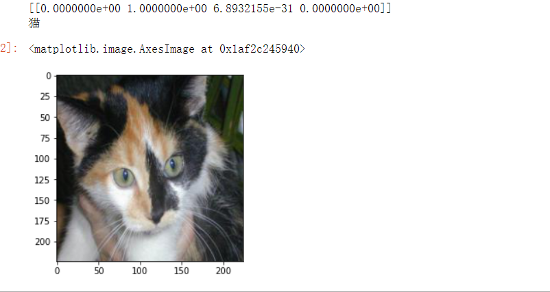
 1 from PIL import Image
 2 def con(file,outdir,w=224,h=224):
 3     img1=Image.open(file)
 4     img2=img1.resize((w,h),Image.BILINEAR)
 5     img2.save(os.path.join(outdir,os.path.basename(file)))
 6 file='D:/python Curriculum design of/forecast/414.jpg'
 7 con(file,'D:/python Curriculum design of/forecast/')
 8 model=load_model('h20')
 9 img_path='D:/python Curriculum design of/forecast/414.jpg'
10 img = load_img(img_path)
11 img = img_to_array(img)
12 img = np.expand_dims(img, axis=0)
13 out = model.predict(img)
14 print(out)
15 dict={'0':'bird','1':'cat','2':'dog','3':'monkey'}
16 for i in range(4):
17     if out[0][i]>0.5:
18         print(dict[str(i)])
19 img=plt.imread('D:/python Curriculum design of/forecast/414.jpg')
20 plt.imshow(img)
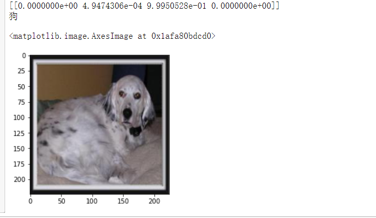
 1 file='D:/python Curriculum design of/forecast/512.jpg'
 2 con(file,'D:/python Curriculum design of/forecast/')
 3 model=load_model('h20')
 4 img_path='D:/python Curriculum design of/forecast/512.jpg'
 5 img = load_img(img_path)
 6 img = img_to_array(img)
 7 img = np.expand_dims(img, axis=0)
 8 out = model.predict(img)
 9 print(out)
10 dict={'0':'bird','1':'cat','2':'dog','3':'monkey'}
11 for i in range(4):
12     if out[0][i]>0.5:
13         print(dict[str(i)])
14 img=plt.imread('D:/python Curriculum design of/forecast/512.jpg')
15 plt.imshow(img)
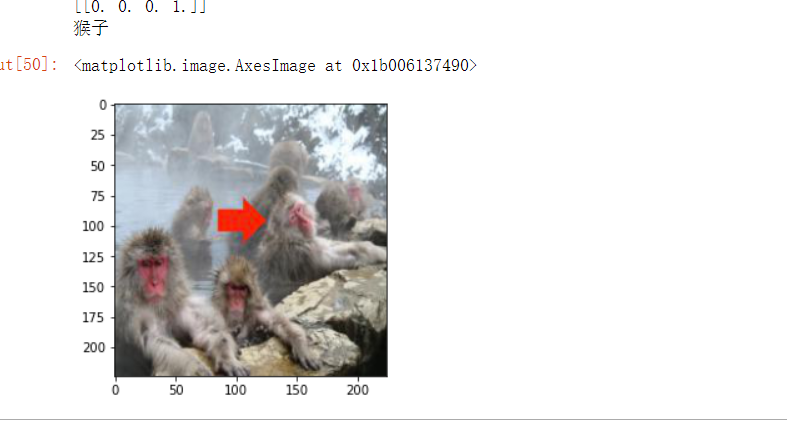
 1 file='D:/python Curriculum design of/forecast/n3044.jpg'
 2 con(file,'D:/python Curriculum design of/forecast/')
 3 model=load_model('h20')
 4 img_path='D:/python Curriculum design of/forecast/n3044.jpg'
 5 img = load_img(img_path)
 6 img = img_to_array(img)
 7 img = np.expand_dims(img, axis=0)
 8 out = model.predict(img)
 9 print(out)
10 dict={'0':'bird','1':'cat','2':'dog','3':'monkey'}
11 for i in range(4):
12     if out[0][i]>0.5:
13         print(dict[str(i)])
14 img=plt.imread('D:/python Curriculum design of/forecast/n3044.jpg')
15 plt.imshow(img)
All codes are attached:
  1 #Import required libraries
  2 import numpy as np
  3 import pandas as pd
  4 import os
  5 import tensorflow as tf
  6 import matplotlib.pyplot as plt
  7 from pathlib import Path
  8 from sklearn.model_selection import train_test_split
  9 from keras.models import Sequential
 10 from keras.layers import Activation
 11 from keras.layers import Dense, Dropout, Flatten, Conv2D, MaxPooling2D
 12 from keras.applications.resnet import preprocess_input
 13 from keras_preprocessing.image import ImageDataGenerator
 14 from keras.models import load_model
 15 from keras.preprocessing.image import load_img, img_to_array
 16 from keras import optimizers
 17
 18 dir = Path('D:/python Curriculum design of/fire')
 19
 20 # use glob Traversal in dir All in path jpg Format and add all file names to the filepaths In the list
 21 filepaths = list(dir.glob(r'**/*.jpg'))
 22
 23 # Separate the divided small file names (category names) in the file and add them to the list of labels
 24 labels = list(map(lambda l: os.path.split(os.path.split(l)[0])[1], filepaths))
 25
 26 # Convert filepaths to Series data type through pandas
 27 filepaths = pd.Series(filepaths, name='FilePaths').astype(str)
 28
 29 # Convert labels to Series data type through pandas
 30 labels = pd.Series(labels, name='Labels').astype(str)
 31
 32 # Synthesize the data types of filepaths and Series into the DataFrame data type
 33 df = pd.merge(filepaths, labels, right_index=True, left_index=True)
 34 df = df[df['Labels'].apply(lambda l: l[-2:] != 'GT')]
 35 df = df.sample(frac=1).reset_index(drop=True)
 36 #View the data of the formed DataFrame
 37 df
 38 #View the image and the corresponding label
 39 fit, ax = plt.subplots(nrows=3, ncols=3, figsize=(10, 7))
 40
 41 for i, a in enumerate(ax.flat):
 42     a.imshow(plt.imread(df.FilePaths[i]))
 43     a.set_title(df.Labels[i])
 44
 45 plt.tight_layout()
 46 plt.show()
 47
 48 # The training set, test set and verification set are generated from the total data set
 49 #Assign the total data to X in a ratio of 10:1_ train, X_ test
 50 X_train, X_test = train_test_split(df, test_size=0.1, stratify=df['Labels'])
 51
 52 print('Shape of Train Data: ', X_train.shape)
 53 print('Shape of Test Data: ', X_test.shape)
 54
 55 # Assign the total data to X in a ratio of 5:1_ train, X_ train
 56 X_train, X_val = train_test_split(X_train, test_size=0.2, stratify=X_train['Labels'])
 57
 58 print('Shape of Train Data: ', X_train.shape)
 59 print('Shape of Val Data: ', X_val.shape)
 60
 61 # View the number of pictures of each label
 62 X_train['Labels'].value_counts(ascending=True)
 63
 64 # Batch size
 65 BATCH_SIZE = 32
 66 # Enter the size of the picture
 67 IMG_SIZE = (224, 224)
 68
 69 # Image preprocessing
 70 img_data_gen = ImageDataGenerator(preprocessing_function=preprocess_input)
 71
 72 X_train = img_data_gen.flow_from_dataframe(dataframe=X_train,
 73                                           x_col='FilePaths',
 74                                           y_col='Labels',
 75                                           target_size=IMG_SIZE,
 76                                           color_mode='rgb',
 77                                           class_mode='binary',
 78                                           batch_size=BATCH_SIZE,
 79                                           seed=42)
 80
 81 X_val = img_data_gen.flow_from_dataframe(dataframe=X_val,
 82                                           x_col='FilePaths',
 83                                           y_col='Labels',
 84                                           target_size=IMG_SIZE,
 85                                           color_mode='rgb',
 86                                           class_mode='binary',
 87                                           batch_size=BATCH_SIZE,
 88                                           seed=42)
 89 X_test = img_data_gen.flow_from_dataframe(dataframe=X_test,
 90                                           x_col='FilePaths',
 91                                           y_col='Labels',
 92                                           target_size=IMG_SIZE,
 93                                           color_mode='rgb',
 94                                           class_mode='binary',
 95                                           batch_size=BATCH_SIZE,
 96                                           seed=42)
 97
 98 #View the processed image and its binary tag
 99 fit, ax = plt.subplots(nrows=2, ncols=3, figsize=(13,7))
100
101 for i, a in enumerate(ax.flat):
102     img, label = X_train.next()
103     a.imshow(img[0],)
104     a.set_title(label[0])
105
106 plt.tight_layout()
107 plt.show()
108
109 #Constructing neural network
110 model = Sequential()
111 # Data normalization processing
112 model.add(tf.keras.layers.experimental.preprocessing.Rescaling(1./255))
113
114 # 1.Conv2D Layer, 32 filters
115 model.add(Conv2D(filters=32, kernel_size=(3,3), padding='same', input_shape=(224, 224, 3)))#The graphics are colored, 'rgb', so set 3
116 model.add(Activation('relu'))
117 model.add(MaxPooling2D(pool_size=(2,2), strides=2, padding='valid'))
118
119 # 2.Conv2D Layer, 64 filters
120 model.add(Conv2D(filters=64, kernel_size=(3,3), padding='same'))
121 model.add(Activation('relu'))
122 model.add(MaxPooling2D(pool_size=(2,2), strides=2, padding='valid'))
123
124 # 3.Conv2D Layer, 128 filters
125 model.add(Conv2D(filters=128, kernel_size=(3,3), padding='same'))
126 model.add(Activation('relu'))
127 model.add(MaxPooling2D(pool_size=(2,2), strides=2, padding='valid'))
128
129 # The data of the input layer is compressed into one-dimensional data, and the full connection layer can only process one-dimensional data
130 model.add(Flatten())
131
132 # Full connection layer
133 model.add(Dense(256))
134 model.add(Activation('relu'))
135
136 # Reduce overfitting
137 model.add(Dropout(0.5))
138
139 # Full connection layer
140 model.add(Dense(1))
141 model.add(Activation('sigmoid'))
142
143 # Model compilation
144 model.compile(optimizer=optimizers.RMSprop(lr=1e-4),
145               loss="categorical_crossentropy",
146               metrics=["accuracy"])
147 #Training model using batch generator
148 h1 = model.fit(X_train, validation_data=X_val,
149                epochs=30, )
150 #Save model
151 model.save('t1')
152
153 #Draw loss curve and accuracy curve
154 accuracy = h1.history['accuracy']
155 loss = h1.history['loss']
156 val_loss = h1.history['val_loss']
157 val_accuracy = h1.history['val_accuracy']
158 plt.figure(figsize=(17, 7))
159 plt.subplot(2, 2, 1)
160 plt.plot(range(30), accuracy,'bo', label='Training Accuracy')
161 plt.plot(range(30), val_accuracy, label='Validation Accuracy')
162 plt.legend(loc='lower right')
163 plt.title('Accuracy : Training vs. Validation ')
164 plt.subplot(2, 2, 2)
165 plt.plot(range(30), loss,'bo' ,label='Training Loss')
166 plt.plot(range(30), val_loss, label='Validation Loss')
167 plt.title('Loss : Training vs. Validation ')
168 plt.legend(loc='upper right')
169 plt.show()
170
171 from PIL import Image
172 def con(file,outdir,w=224,h=224):
173     img1=Image.open(file)
174     img2=img1.resize((w,h),Image.BILINEAR)
175     img2.save(os.path.join(outdir,os.path.basename(file)))
176 file='D:/python Curriculum design / NA_Fish_Dataset/Black Sea Sprat/F_23.jpg'
177 con(file,'D:/python Curriculum design / NA_Fish_Dataset/Black Sea Sprat/')
178 model=load_model('t1')
179 img_path='D:/python Curriculum design / NA_Fish_Dataset/Black Sea Sprat/F_23.jpg'
180 img = load_img(img_path)
181 img = img_to_array(img)
182 img = np.expand_dims(img, axis=0)
183 out = model.predict(img)
184 if out[0]>0.5:
185         print('The probability of fire is',out[0])
186 else:
187          print('Not a fire')
188 img=plt.imread('D:/python Curriculum design / NA_Fish_Dataset/Black Sea Sprat/F_23.jpg')
189 plt.imshow(img)
190
191 dir = Path('D:/python Curriculum design 1')
192
193 # Use glob to traverse all jpg files in the dir path, and add all file names to the file paths list
194 filepaths = list(dir.glob(r'**/*.jpg'))
195
196 # Separate the divided small file name (category name) in the file and add it to the labels In the list of
197 labels = list(map(lambda l: os.path.split(os.path.split(l)[0])[1], filepaths))
198
199 # take filepaths adopt pandas Convert to Series data type
200 filepaths = pd.Series(filepaths, name='FilePaths').astype(str)
201
202 # take labels adopt pandas Convert to Series data type
203 labels = pd.Series(labels, name='Labels').astype(str)
204
205 # take filepaths and Series Two Series Data type composition for DataFrame data type
206 df = pd.merge(filepaths, labels, right_index=True, left_index=True)
207 df = df[df['Labels'].apply(lambda l: l[-2:] != 'GT')]
208 df = df.sample(frac=1).reset_index(drop=True)
209
210 #Constructing neural network
211 model = Sequential()
212 # Data normalization processing
213 model.add(tf.keras.layers.experimental.preprocessing.Rescaling(1./255))
214
215 # 1.Conv2D Layer, 32 filters
216 model.add(Conv2D(filters=32, kernel_size=(3,3), padding='same', input_shape=(224, 224, 3)))#The graphics are color,'rgb',So set 3
217 model.add(Activation('relu'))
218 model.add(MaxPooling2D(pool_size=(2,2), strides=2, padding='valid'))
219
220 # 2.Conv2D Layer, 64 filters
221 model.add(Conv2D(filters=64, kernel_size=(3,3), padding='same'))
222 model.add(Activation('relu'))
223 model.add(MaxPooling2D(pool_size=(2,2), strides=2, padding='valid'))
224
225 # 3.Conv2D Layer, 128 filters
226 model.add(Conv2D(filters=128, kernel_size=(3,3), padding='same'))
227 model.add(Activation('relu'))
228 model.add(MaxPooling2D(pool_size=(2,2), strides=2, padding='valid'))
229
230 # The data of the input layer is compressed into one-dimensional data, and the full connection layer can only process one-dimensional data
231 model.add(Flatten())
232
233 # Full connection layer
234 model.add(Dense(256))
235 model.add(Activation('relu'))
236
237 # Reduce overfitting
238 model.add(Dropout(0.5))
239
240 # Full connection layer
241 model.add(Dense(4))#There are four categories to be identified
242 model.add(Activation('softmax'))#softmax It is based on binary classification function sigmoid Multi classification function
243
244 # Model compilation
245 model.compile(optimizer=optimizers.RMSprop(lr=1e-4),
246               loss="categorical_crossentropy",
247               metrics=["accuracy"])
248 #Training model using batch generator
249 h1 = model.fit(X_train, validation_data=X_val,
250                epochs=30, )
251 #Save model
252 model.save('h21')
253
254
255 #Draw loss curve and accuracy curve
256 accuracy = h1.history['accuracy']
257 loss = h1.history['loss']
258 val_loss = h1.history['val_loss']
259 val_accuracy = h1.history['val_accuracy']
260 plt.figure(figsize=(17, 7))
261 plt.subplot(2, 2, 1)
262 plt.plot(range(30), accuracy,'bo', label='Training Accuracy')
263 plt.plot(range(30), val_accuracy, label='Validation Accuracy')
264 plt.legend(loc='lower right')
265 plt.title('Accuracy : Training vs. Validation ')
266 plt.subplot(2, 2, 2)
267 plt.plot(range(30), loss,'bo' ,label='Training Loss')
268 plt.plot(range(30), val_loss, label='Validation Loss')
269 plt.title('Loss : Training vs. Validation ')
270 plt.legend(loc='upper right')
271 plt.show()
272
273 #definition ImageDataGenerator parameter
274 train_datagen = ImageDataGenerator(rescale=1./255,
275                                   rotation_range=40, #Rotate the image randomly by 40 degrees
276                                   width_shift_range=0.2, #The translation scale in the horizontal direction is 0.2
277                                   height_shift_range=0.2, #The translation scale in the vertical direction is 0.2
278                                   shear_range=0.2, #The angle of random staggered transformation is 0.2
279                                   zoom_range=0.2, #The range of random scaling of the picture is 0.2
280                                   horizontal_flip=True, #Randomly flip half the image horizontally
281                                   fill_mode='nearest') #Fill create pixels
282
283 X_val1 = ImageDataGenerator(rescale=1./255)
284
285 X_train1 = train_datagen.flow_from_dataframe(
286                         X_train,
287                         target_size=(150,150),
288                         batch_size=32,
289                         class_mode='categorical'
290                         )
291
292 X_val1= test_datagen.flow_from_dataframe(
293                         X_test,
294                         target_size=(150,150),
295                         batch_size=32,
296                         class_mode='categorical')
297
298 from PIL import Image
299 def con(file,outdir,w=224,h=224):
300     img1=Image.open(file)
301     img2=img1.resize((w,h),Image.BILINEAR)
302     img2.save(os.path.join(outdir,os.path.basename(file)))
303 file='D:/python Curriculum design of/forecast/414.jpg'
304 con(file,'D:/python Curriculum design of/forecast/')
305 model=load_model('h21')
306 img_path='D:/python Curriculum design of/forecast/414.jpg'
307 img = load_img(img_path)
308 img = img_to_array(img)
309 img = np.expand_dims(img, axis=0)
310 out = model.predict(img)
311 print(out)
312 dict={'0':'bird','1':'cat','2':'dog','3':'monkey'}
313 for i in range(4):
314     if out[0][i]>0.5:
315         print(dict[str(i)])
316 img=plt.imread('D:/python Curriculum design of/forecast/414.jpg')
317 plt.imshow(img)
(4) Summary: the main content of this program design is the label learning of machine learning. Through this course design, I have deepened my understanding of machine learning and its label learning.
Machine learning is a method of using data, training models, and then model prediction. This study is mainly to practice two classification and multi classification. Secondary classification: the secondary classification function used is sigmoid, while the multi classification function used by softmax based on secondary classification. Sigmoid is used to nonlinearize each output value, while sofmax is used to calculate the specific gravity. The results of the two are similar and have the function of normalization. However, softmax is a process of normalization for the output result, and sigmoid is a nonlinear activation process, that is, when the output layer is a divine element, sigmoid will be used. Softmax is generally used in combination with one hot tag, It is generally used in the last layer of the network. Sigmoid is used with 0,1 real tags. When using softmax, the loss function should be set to categorical_ Crossintropy loss function, and when sigmoid is used, the loss function is set to binary_crossentropy loss function.
The deficiency of this program design: the effect of data enhancement is not very obvious, and the image distortion is encountered in the design process, resulting in the slow rise of training accuracy