Hierarchical Clustering (Partition Clustering)

Clustering refers to a large number of unknown labeled datasets, which are divided into several different categories according to the data characteristics existing inside the data, so that the data within the categories are similar, and the data similarity between the categories is small; it belongs to unsupervised learning.

Algorithmic steps

1. Initialized k centers

2. Assign categories to each sample based on distance

3. Update the center point of each category (update to the mean of all samples in that category)

4. Repeat the above two steps until a termination condition is reached

 

Hierarchical clustering decomposes a given dataset hierarchically until a certain condition is met. Traditional hierarchical clustering algorithms are divided into two main categories:

Aggregated Hierarchical Clustering

The AGNES algorithm==>uses a bottom-up strategy.

Each object is initially treated as a cluster, and then these clusters are merged step by step according to some criteria (the measure of similarity between the two clusters). The distance between the two clusters can be determined by the similarity of the nearest data points in the two different clusters. The merging process of the clusters is repeated until all the objects are full.Number of foot clusters.

AGNES is to group each fruit into a category.

 

Selection of merge points:

• Maximum distance between two clusters (complete)

• Minimum distance between two clusters (word)

• average distance between two clusters

For chain clustering, bar clustering is better.

Code:

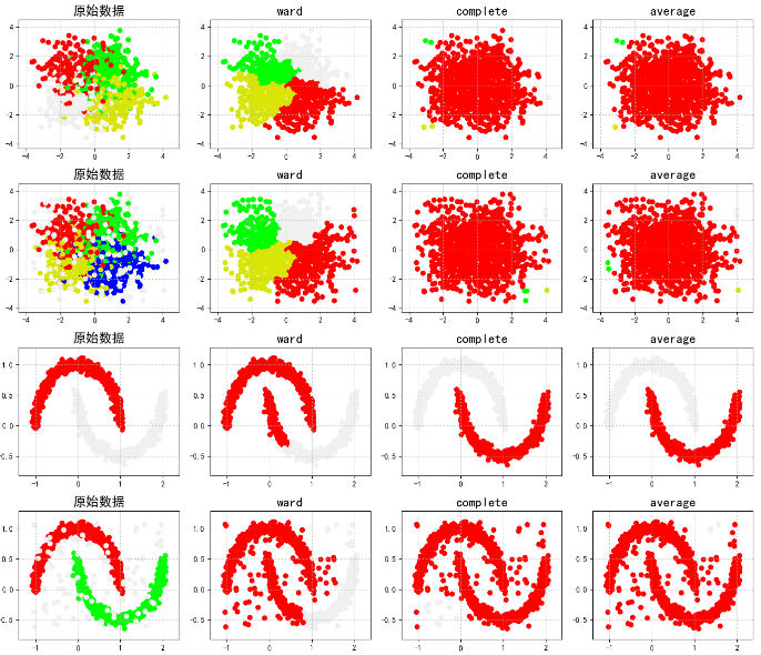
linkages : complete,word,average

import numpy as np
import matplotlib as mpl
import matplotlib.pyplot as plt
# call AGNES
from sklearn.cluster import AgglomerativeClustering
from sklearn.neighbors import kneighbors_graph  ## K-Nearest Neighbor Calculation for KNN
import sklearn.datasets as ds
# Intercept exception information
import warnings
​
warnings.filterwarnings('ignore')
# Set properties to prevent Chinese scrambling
mpl.rcParams['font.sans-serif'] = [u'SimHei']
mpl.rcParams['axes.unicode_minus'] = False
# Analog data generation: Generate 600 pieces of data
np.random.seed(0)
n_clusters = 4
N = 1000
data1, y1 = ds.make_blobs(n_samples=N, n_features=2, centers=((-1, 1), (1, 1), (1, -1), (-1, -1)), random_state=0)
​
n_noise = int(0.1 * N)
r = np.random.rand(n_noise, 2)
min1, min2 = np.min(data1, axis=0)
max1, max2 = np.max(data1, axis=0)
r[:, 0] = r[:, 0] * (max1 - min1) + min1
r[:, 1] = r[:, 1] * (max2 - min2) + min2
​
data1_noise = np.concatenate((data1, r), axis=0)
y1_noise = np.concatenate((y1, [4] * n_noise))
# Fitting crescent data
data2, y2 = ds.make_moons(n_samples=N, noise=.05)
data2 = np.array(data2)
n_noise = int(0.1 * N)
r = np.random.rand(n_noise, 2)
min1, min2 = np.min(data2, axis=0)
max1, max2 = np.max(data2, axis=0)
r[:, 0] = r[:, 0] * (max1 - min1) + min1
r[:, 1] = r[:, 1] * (max2 - min2) + min2
data2_noise = np.concatenate((data2, r), axis=0)
y2_noise = np.concatenate((y2, [3] * n_noise))
​
​
def expandBorder(a, b):
    d = (b - a) * 0.1
    return a - d, b + d
​
​
## Drawing
# Given the color of the drawing
cm = mpl.colors.ListedColormap(['#FF0000', '#00FF00', '#0000FF', '#d8e507', '#F0F0F0'])
plt.figure(figsize=(14, 12), facecolor='w')
linkages = ("ward", "complete", "average")  # Put several distance methods list Inside, back direct loop
for index, (n_clusters, data, y) in enumerate(((4, data1, y1), (4, data1_noise, y1_noise),
                                               (2, data2, y2), (2, data2_noise, y2_noise))):
    # The first two four represent rows and columns, and the third parameter represents the number of subgraphs(From 1, left to right)
    plt.subplot(4, 4, 4 * index + 1)
    plt.scatter(data[:, 0], data[:, 1], c=y, cmap=cm)
    plt.title(u'Raw data', fontsize=17)
    plt.grid(b=True, ls=':')
    min1, min2 = np.min(data, axis=0)
    max1, max2 = np.max(data, axis=0)
    plt.xlim(expandBorder(min1, max1))
    plt.ylim(expandBorder(min2, max2))
​
    # Calculate the distance between categories(Calculate distances for only the closest seven samples) -- Hope agens In the algorithm, the distance between points is calculated without repetition
    connectivity = kneighbors_graph(data, n_neighbors=7, mode='distance', metric='minkowski', p=2, include_self=True)
    connectivity = (connectivity + connectivity.T)
    for i, linkage in enumerate(linkages):
        ##Modeling and passing values
        ac = AgglomerativeClustering(n_clusters=n_clusters, affinity='euclidean',
                                     connectivity=connectivity, linkage=linkage)
        ac.fit(data)
        y = ac.labels_
​
        plt.subplot(4, 4, i + 2 + 4 * index)
        plt.scatter(data[:, 0], data[:, 1], c=y, cmap=cm)
        plt.title(linkage, fontsize=17)
        plt.grid(b=True, ls=':')
        plt.xlim(expandBorder(min1, max1))
        plt.ylim(expandBorder(min2, max2))
​
plt.tight_layout(0.5, rect=(0, 0, 1, 0.95))
plt.show()

AGNES uses the results of different merges:

 

 

Split hierarchical clustering (similar to decision trees)

DIANA algorithm==>uses a top-down strategy.

All objects are first placed in a cluster, then subdivided into smaller and smaller clusters according to a set rule (e.g. by kmeans) until an end condition (the number of clusters or the distance between clusters reaches a threshold) is reached.

1, place all sample data as a cluster in a queue 2, divide it into two subclusters (initialize two center points for clustering), add the subclusters to the queue 3, iterate through the second step until the termination condition is reached (number of clusters, minimum square error, number of iterations)

Selection of Split Points:

• Error of each cluster

• SE for each cluster (preferring this strategy)

• Select the cluster with the largest amount of sample data

DIANA is similar to breaking bread

 

AGNES and DIANA

• Simple, easy to understand

• Merge/split point selection is not easy

• The merge/categorization operation cannot be undone (bread cut cannot close)

• Large datasets are not suitable

• Less efficient O(t*n2), t is the number of iterations, n is the number of sample points

Optimization of AGNES

BIRCH (Master)

BIRCH algorithm (balanced iterative reduction clustering):

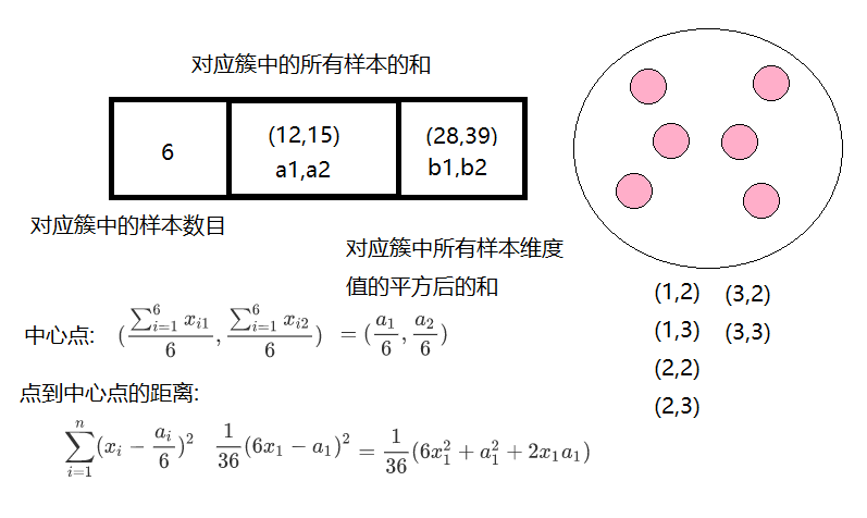
Cluster features use three tuples to carry out information about a cluster, and cluster features are computed by constructing a cluster feature tree that satisfies the restrictions of the branching factor and cluster diameter. A cluster feature tree is actually a height balance tree with two parameters, the branching factor specifies the maximum number of children at each node of the tree.The class diameter reflects the distance range to such points; the non-leaf node is the maximum eigenvalue of its children;

Triple

 

Construction of BIRCH

 

 

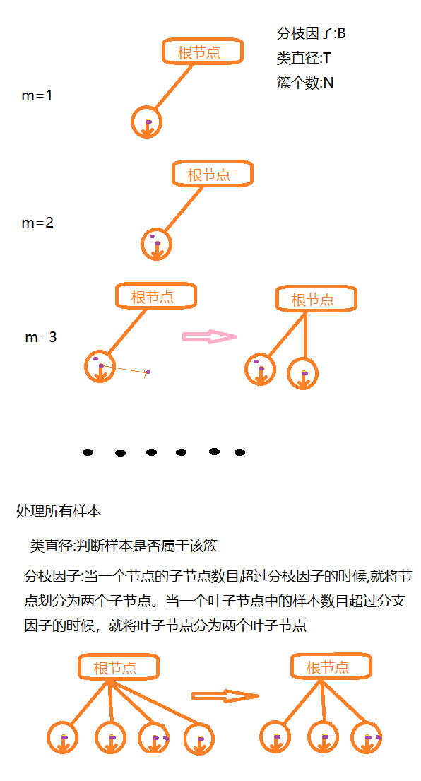
Judging from the root node to the leaf node one level at a time,

Advantages and disadvantages:

• Suitable for large-scale datasets, linear efficiency;

• Suitable only for datasets with convex or spherical distribution, requiring a given number of clusters and correlation parameters between clusters

Code implementation:

Library parameters:

1. threshold class diameter

2. branshing_factor branching factor

3. Number of n_clusters

from itertools import cycle
from time import time
import numpy as np
import matplotlib as mpl
import matplotlib.pyplot as plt
import matplotlib.colors as colors
​
from sklearn.cluster import Birch
from sklearn.datasets.samples_generator import make_blobs
​
## Set properties to prevent Chinese scrambling
mpl.rcParams['font.sans-serif'] = [u'SimHei']
mpl.rcParams['axes.unicode_minus'] = False
## Generate analog data
xx = np.linspace(-22, 22, 10)
yy = np.linspace(-22, 22, 10)
xx, yy = np.meshgrid(xx, yy)
n_centres = np.hstack((np.ravel(xx)[:, np.newaxis],
                       np.ravel(yy)[:, np.newaxis]))
# The resulting 100,000 feature attributes are 2 and the category is 100,Datasets with a Gaussian distribution
X, y = make_blobs(n_samples=100000, n_features=2, centers=n_centres, random_state=28)
# Create different parameters (cluster diameter) Birch hierarchical clustering
birch_models = [
    Birch(threshold=1.7, n_clusters=None),
    Birch(threshold=0.5, n_clusters=None),
    Birch(threshold=1.7, n_clusters=100)
]
# threshold: Threshold of cluster diameter,    branching_factor: Number of large leaves
​
# We can also add parameters to try the effect, such as adding a branching factor branching_factor，Given different parameter values, see the results of clustering
## Drawing
final_step = [u'diameter=1.7;n_lusters=None', u'diameter=0.5;n_clusters=None', u'diameter=1.7;n_lusters=100']
​
plt.figure(figsize=(12, 8), facecolor='w')
plt.subplots_adjust(left=0.02, right=0.98, bottom=0.1, top=0.9)
colors_ = cycle(colors.cnames.keys())
cm = mpl.colors.ListedColormap(colors.cnames.keys())
​
for ind, (birch_model, info) in enumerate(zip(birch_models, final_step)):
    t = time()
    birch_model.fit(X)
    time_ = time() - t
    # Get model results ( label And center point)
    labels = birch_model.labels_
    centroids = birch_model.subcluster_centers_
    n_clusters = len(np.unique(centroids))
    print("Birch Algorithm, parameter information is:%s；Modeling takes time to build:%.3f Seconds; number of cluster centers:%d" % (info, time_, len(np.unique(labels))))
​
    # Drawing
    subinx = 221 + ind
    plt.subplot(subinx)
    for this_centroid, k, col in zip(centroids, range(n_clusters), colors_):
        mask = labels == k
        plt.plot(X[mask, 0], X[mask, 1], 'w', markerfacecolor=col, marker='.')
        if birch_model.n_clusters is None:
            plt.plot(this_centroid[0], this_centroid[1], '*', markerfacecolor=col, markeredgecolor='k', markersize=2)
    plt.ylim([-25, 25])
    plt.xlim([-25, 25])
    plt.title(u'Birch algorithm%s，time consuming%.3fs' % (info, time_))
    plt.grid(False)
​
# Original Dataset Display
plt.subplot(224)
plt.scatter(X[:, 0], X[:, 1], c=y, s=1, cmap=cm, edgecolors='none')
plt.ylim([-25, 25])
plt.xlim([-25, 25])
plt.title(u'Raw data')
plt.grid(False)
​
plt.show()

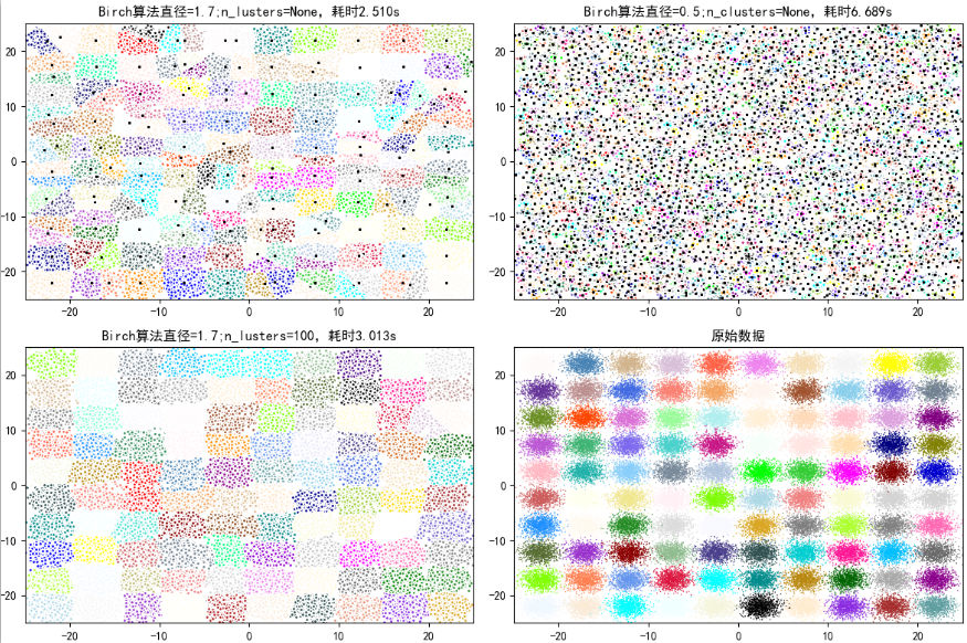
Run result:

Birch Algorithm, parameter information is: diameter=1.7;n_lusters=None；Modeling takes time to build:2.510 Seconds; number of cluster centers:171Birch Algorithm, parameter information is: diameter=0.5;n_clusters=None；Modeling takes time to build:6.689 Seconds; number of cluster centers:3205Birch Algorithm, parameter information is: diameter=1.7;n_lusters=100；Modeling takes time to build:3.013 Seconds; number of cluster centers:100

Process finished with exit code 0

 

CURE (unused)

CURE algorithm (using clustering on behalf of points):

The algorithm considers each data point as a class, then merges the closest classes until the required number of classes is reached.However, the difference with the AGNES algorithm is that all points are cancelled or a class is represented by a center point + distance

Instead, a fixed number of well-distributed points are selected from each class as representative points of this class, and these representative points are multiplied by an appropriate shrinking factor to make them closer to the class center point.

The shrinkage characteristics of the representative points can adjust the model to match those non-spherical scenes, and the use of the shrinkage factor can reduce the impact of noise on clustering.

 

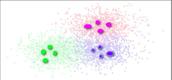
Find several special points to replace the samples in the entire category

Advantages and disadvantages: Random sampling and partitioning can improve the efficiency of algorithm execution in application scenarios that can handle non-spherical distribution