1. General
1.1 how does the decision tree work
Decision Tree is a nonparametric supervised learning method. It can summarize decision rules from a series of characteristic and labeled data, and present these rules with the structure of tree view to solve the problems of classification and regression.
Decision tree algorithm is easy to understand, suitable for all kinds of data, and has good performance in solving all kinds of problems. In particular, various integration algorithms with tree model as the core are widely used in various industries and fields.
The essence of decision tree algorithm is a graph structure. We only need to ask a series of questions
According to the classification.
For example, let's take a look at the following data set, which is the data of a series of known species and their categories:
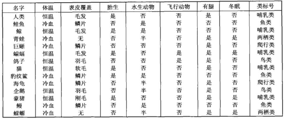
The goal now is to divide animals into mammals and non mammals. According to the collected data, the decision tree algorithm calculates the following decision tree for us:
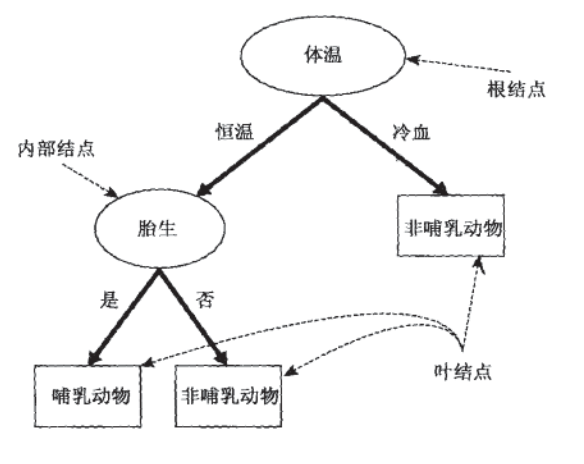
If a new species Python is found, it is cold-blooded, with scales on its body surface, and it is not viviparous, we can judge its category through this decision tree.
In this decision-making process, we have been asking questions about the characteristics of records. The place where the initial problem is located is called the root node. Every problem before reaching a conclusion is an intermediate node, and every conclusion (animal category) is called a leaf node.
Key concept: node
(1) Root node: there are no in edges and out edges. Include initial, feature specific questions.
(2) Intermediate node: there are both incoming and outgoing edges. There is only one incoming edge and many outgoing edges. Are questions about characteristics.
(3) Leaf node: there are in edges but no out edges. Each leaf node is a category label.
(4) Child node and parent node: among the two connected nodes, the parent node is closer to the root node, and the other is the child node.
The core of decision tree algorithm is to solve two problems:
(1) How to find the best node and branch from the data table?
(2) How to stop the growth of decision tree and prevent over fitting?
1.2 decision tree in sklearn
[1] Module sklearn.tree
The classes of decision trees in sklearn are all under the "tree" module. This module contains five classes in total:
| english | chinese |
|---|---|
| tree.DecisionTreeClassifier | Classification tree |
| tree.DecisionTreeRegressor | Regression tree |
| tree.export_graphviz | The generated decision tree is exported to DOT format for drawing |
| tree.ExtraTreeClassifier | High random version classification tree |
| tree.ExtraTreeRegressor | High random version of regression tree |
[2] Basic modeling process of sklearn
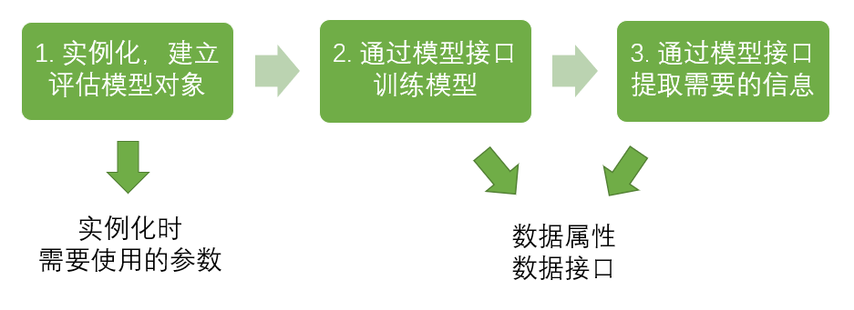
In this process, the corresponding code of the classification tree is:
from sklearn import tree #Import required modules
clf = tree.DecisionTreeClassifier()   #instantiation
clf = clf.fit(X_train,y_train) #Training model with training set data
result = clf.score(X_test,y_test) #Import the test set and call the required information from the interface.
2. DecisionTreeClassifier and red wine dataset
class sklearn.tree.DecisionTreeClassifier (
					criterion='gini',
					splitter='best',
					max_depth=None,
					min_samples_split=2,
					min_samples_leaf=1,
					min_weight_fraction_leaf=0.0,
					max_features=None,
					random_state=None,
					max_leaf_nodes=None,
					min_impurity_decrease=0.0,
					min_impurity_split=None,
					class_weight=None,
					presort=False)
2.1 important parameters
2.1.1 criterion
In order to transform the table into a tree, the decision tree needs to find the best node and the best branching method. For the classification tree, the index to measure this "best" is called "impure" Generally speaking, the lower the impurity, the better the fitting of the decision tree to the training set. The core of the decision tree algorithm used now is mostly around the optimization of a certain impurity related index.
Impure: Gini impure refers to the expected error rate of a data item when a result from the set is randomly applied to the set. It roughly means the probability that a random event becomes its opposite event.
Impure is calculated based on nodes. Each node in the tree will have an impure, and the impure of child nodes must be lower than that of parent nodes, that is, on the same decision tree, the impure of leaf nodes must be the lowest.
The Criterion parameter is used to determine the calculation method of impurity. sklearn provides two options:
1)"Input" entropy",Using information entropy( Entropy)
2)"Input" gini",Use Gini coefficient( Gini Impurity)
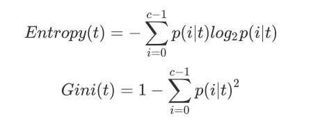
Where t represents a given node, i represents any label classification, and represents the proportion of label classification i in node t. note that when using information entropy, sklearn actually calculates the information gain based on information entropy, that is, the difference between the information entropy of the parent node and the information entropy of the child node.
Compared with Gini coefficient, information entropy is more sensitive to impurity, and the punishment for impurity is the strongest. However, in practical use, the effects of information entropy and Gini coefficient are basically the same. The calculation of information entropy is slower than that of Gini coefficient, because the calculation of Gini coefficient does not involve logarithm. In addition, because information entropy is more sensitive to impurity, when information entropy is used as an index, the decision tree The growth of the model will be more "fine". Therefore, for high-dimensional data or data with a lot of noise, the information entropy is easy to over fit, and the Gini coefficient often has a better effect in this case. When the model fitting degree is insufficient, that is, when the model does not show well in both the training set and the test set, the information entropy is used. Of course, these are not absolute.
| parameter | criterion |
|---|---|
| How does it affect the model? | Determine the calculation method of impure to help find the best node and branch. The lower the impure, the better the fitting of the decision tree to the training set |
| What are the possible inputs? | Do not fill in the default gini coefficient, fill in gini to use gini coefficient, and fill in entropy to use information gain |
| How to select parameters? | Usually, Gini coefficient is used. The data dimension is large. When the noise is large, the Gini coefficient dimension is low. When the data is clear, there is no difference between information entropy and Gini coefficient. When the fitting degree of decision tree is not enough, try using both information entropy. If not, change the other one |
The basic process of decision tree can be summarized as follows:

Until no more features are available or the overall impurity index is optimal, the decision tree will stop growing.
Example: build a tree
1. Import the required algorithm libraries and modules
from sklearn import tree
from sklearn.datasets import load_wine
from sklearn.model_selection import train_test_split
2. Explore data
wine = load_wine()
print(wine.data.shape)
print(wine.target)

#If wine is a table, it should look like this
import pandas as pd
pd.concat([pd.DataFrame(wine.data), pd.DataFrame(wine.target)], axis=1)
print(wine.feature_names)
print(wine.target_names)
3. It is divided into training set and test set
Xtrain, Xtest, Ytrain, Ytest = train_test_split(wine.data,wine.target,test_size=0.3)
print(Xtrain.shape)
print(Xtest.shape)
4. Establish model
clf = tree.DecisionTreeClassifier(criterion="entropy")
clf = clf.fit(Xtrain, Ytrain)
score = clf.score(Xtest, Ytest) #Returns the accuracy of the forecast
print(score)
5. Draw a tree
feature_name = ['alcohol','malic acid','ash','Alkalinity of ash','magnesium','Total phenol','flavonoid','Non flavane phenols','anthocyanin',
                'Color intensity','tone','od280/od315 Diluted wine','proline']
import graphviz

dot_data = tree.export_graphviz(
    clf,
    out_file=None,
    feature_names=feature_name,
    class_names=["Gin","Shirley","Belmord"],
    filled=True,
    rounded=True
)
# Remove Chinese garbled Code: dot_data. Replace ('helvetica ',' Microsoft YaHei '), encoding ='utf-8'
graph = graphviz.Source(dot_data.replace('helvetica','"Microsoft YaHei"'), encoding='utf-8')
graph.view()
6. Explore the decision tree
#Feature importance. (feature, importance)
print(clf.feature_importances_)
print([*zip(feature_name,clf.feature_importances_)])
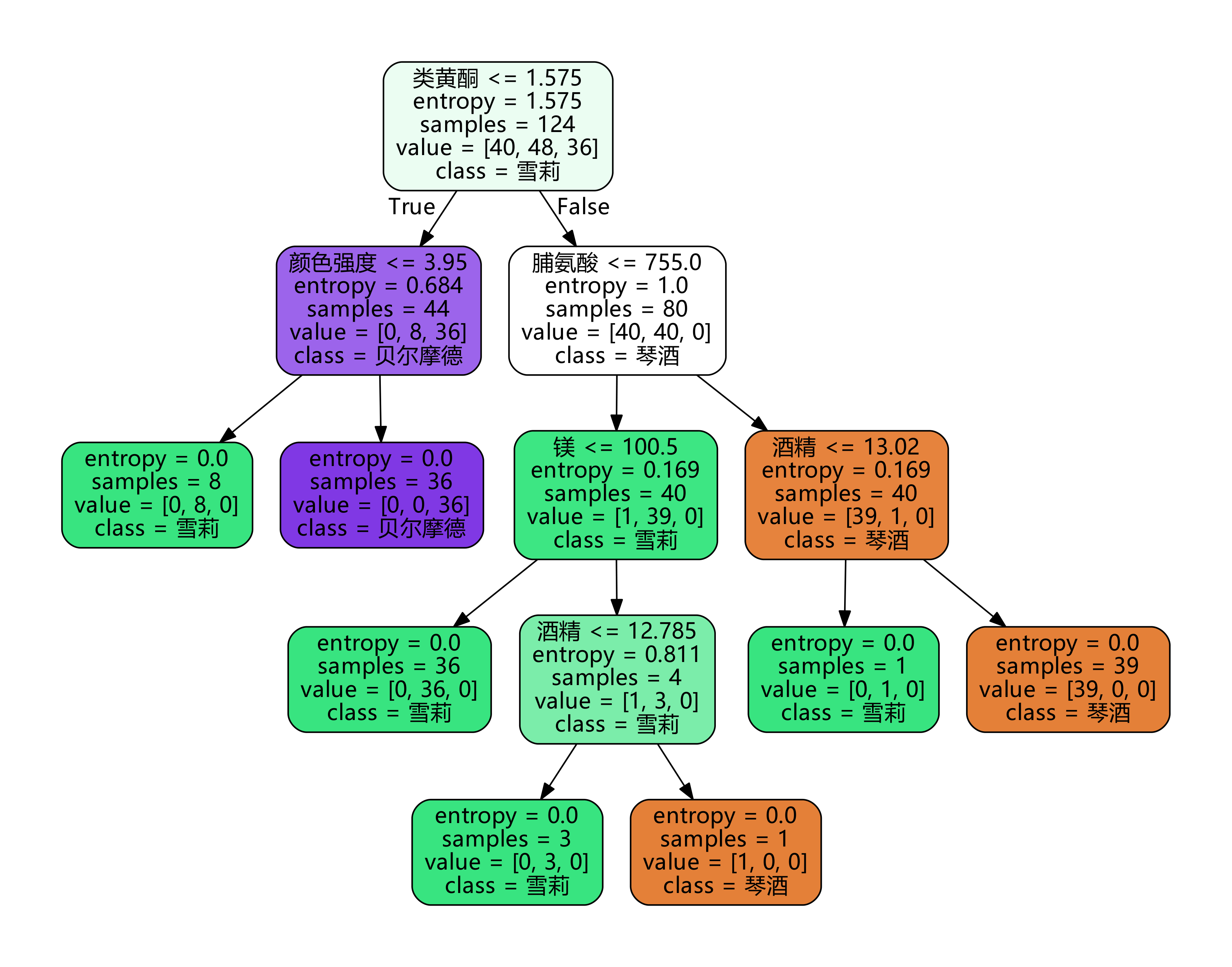
We have established a complete decision tree with only one parameter. However, when we go back to step 4 to establish the model, the score will fluctuate around a certain value, causing each tree drawn in step 5 to be different. Why is it unstable? Will it be unstable if other data sets are used?
As we mentioned before, no matter how the decision tree model evolves, the essence of branching still pursues the optimization of an index related to impurity. As we mentioned, impurity is calculated based on nodes, that is, when building a tree, the decision tree pursues an optimized tree by optimizing nodes, but can the optimal node ensure the optimal tree? The integration algorithm is used to solve this problem: sklearn says that since a tree cannot guarantee the optimization, it is necessary to build more different trees and then choose the best one. How to build different trees from a set of data sets? In each branching, instead of using all the features, some features are randomly selected, and the node with the best impurity related index is selected as the node for branching. In this way, the tree generated each time will be different.
2.1.2 random_state & splitter
random_state is used to set the parameter of the random pattern in the branch. The default is None. The randomness will be more obvious in the high dimension, and the randomness will hardly appear in the low dimension data (such as iris data set). If you enter any integer, the same tree will grow all the time to stabilize the model. The splitter is also used to control the random options in the decision tree. There are two input values: enter "best". Although the decision tree branches randomly, it will give priority to the more important features for branching (the importance can be viewed through the attribute feature_imports_), and enter "random" , the decision tree will be more random when branching. The tree will be deeper and larger because it contains more unnecessary information, and the fitting of the training set will be reduced due to these unnecessary information. This is also a way to prevent over fitting. When you predict that your model will be over fitted, use these two parameters to help you reduce the possibility of over fitting after the tree is built. Of course, once the tree is built, We still use pruning parameters to prevent over fitting.
clf = tree.DecisionTreeClassifier(criterion="entropy",random_state=30,splitter="random")
clf = clf.fit(Xtrain, Ytrain)
score = clf.score(Xtest, Ytest) #Returns the accuracy of the forecast
print(score)

feature_name = ['alcohol','malic acid','ash','Alkalinity of ash','magnesium','Total phenol','flavonoid','Non flavane phenols','anthocyanin',
                'Color intensity','tone','od280/od315 Diluted wine','proline']
import graphviz
dot_data = tree.export_graphviz(
    clf,
    feature_names=feature_name,
    class_names=["Gin","Shirley","Belmord"],
    filled=True,
    rounded=True
)
# Remove Chinese garbled Code: dot_data. Replace ('helvetica ',' Microsoft YaHei '), encoding ='utf-8'
graph = graphviz.Source(dot_data.replace('helvetica','"Microsoft YaHei"'), encoding='utf-8')
graph.view()
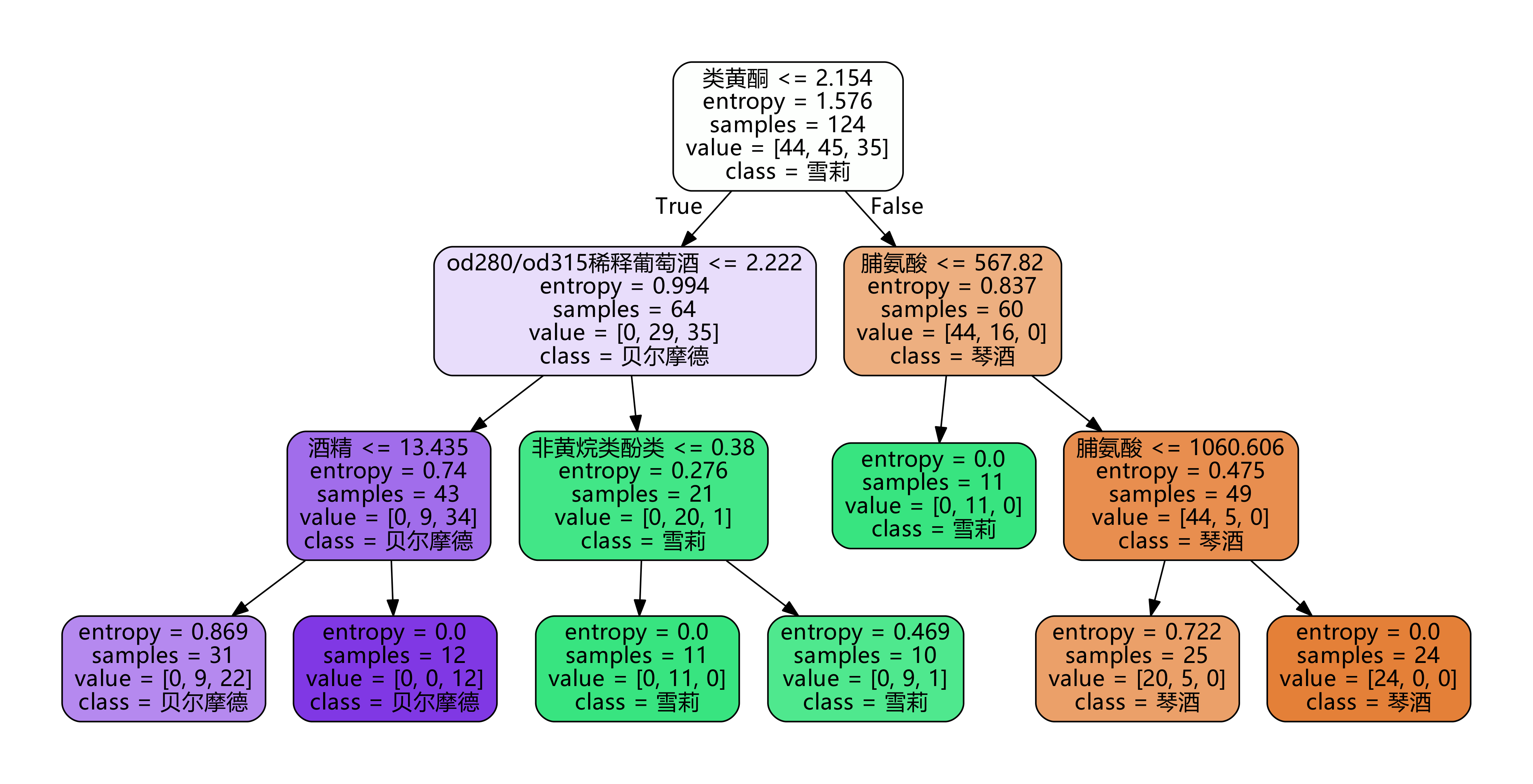
2.1.3 pruning parameters
Without restrictions, a decision tree will grow until the index to measure the purity is the best, or no more features are available. Such a decision tree will often be over fitted, that is, it will perform well in the training set but poorly in the test set. The sample data we collect cannot be completely consistent with the overall situation, so when a decision tree The rules it finds must contain the noise in the training samples, and its fitting degree to the unknown data is insufficient.
#How well does our tree fit the training set?
score_train = clf.score(Xtrain, Ytrain)
score_train # The result is 1.0
In order to make the decision tree more generalized, we should prune the decision tree. Pruning strategy has a great impact on the decision tree, and the correct pruning strategy is the core of optimizing the decision tree algorithm.
sklearn provides us with different pruning strategies:
[1]max_depth
Limit the maximum depth of the tree and cut off all branches exceeding the set depth
This is the most widely used pruning parameter, which is very effective in high dimensions and low sample size. If the decision tree grows one more layer, the demand for sample size will double, so limiting the tree depth can effectively limit over fitting. It is also very practical in the integration algorithm. In practical use, it is recommended to start with = 3, see the fitting effect, and then decide whether to increase the set depth.
[2]min_samples_leaf & min_samples_split
Min_samples_leaf defines that each child node of a node after branching must contain at least min_samples_leaf training samples, otherwise branching will not occur, or branching will occur in the direction that each child node contains min_samples_leaf samples
It is generally used in combination with max_depth. It has a magical effect in the regression tree and can make the model smoother. Setting the number of this parameter too small will cause over fitting, and setting it too large will prevent the model from learning data. Generally speaking, it is recommended to start with = 5. If the sample size contained in the leaf node changes greatly, it is recommended to enter floating-point numbers as the percentage of the sample size At the same time, this parameter can ensure the minimum size of each leaf and avoid the occurrence of low variance and over fitting leaf nodes in regression problems. For classification problems with few categories, = 1 is usually the best choice.
Min_samples_split limits that a node must contain at least min_samples_split training samples before it can be branched, otherwise branching will not occur.
import graphviz
feature_name = ['alcohol','malic acid','ash','Alkalinity of ash','magnesium','Total phenol','flavonoid','Non flavane phenols','anthocyanin',
                'Color intensity','tone','od280/od315 Diluted wine','proline']
clf = tree.DecisionTreeClassifier(criterion="entropy"
                                ,random_state=30
                                ,splitter="random"
                                ,max_depth=3
                                ,min_samples_leaf=10
                                ,min_samples_split=10
                                )

clf = clf.fit(Xtrain, Ytrain)
dot_data = tree.export_graphviz(clf
                                ,feature_names= feature_name
                                ,class_names=["Gin","Shirley","Belmord"]
                                ,filled=True
                                ,rounded=True
                                )
# Remove Chinese garbled Code: dot_data. Replace ('helvetica ',' Microsoft YaHei '), encoding ='utf-8'
graph = graphviz.Source(dot_data.replace('helvetica','"Microsoft YaHei"'), encoding='utf-8')
graph.view()
[3] Confirm the optimal pruning parameters
Then how to determine what value to fill in for each parameter? At this time, we will use the curve to determine the superparameter to judge, and continue to use the decision tree model clf we have trained. The learning curve of superparameter is a curve with the value of superparameter as the horizontal benchmark and the measurement index of the model as the vertical coordinate. It is used to measure the value of different superparameters The performance line of the model. In our built decision tree, our model metric is score.
import matplotlib.pyplot as plt
test = []
for i in range(10):
    clf = tree.DecisionTreeClassifier(max_depth=i+1
                                    ,criterion="entropy"
                                    ,random_state=30
                                    ,splitter="random"
                                    )
    clf = clf.fit(Xtrain, Ytrain)
    score = clf.score(Xtest, Ytest)
    test.append(score)
plt.plot(range(1,11),test,color="red",label="max_depth")
plt.legend()
plt.show()
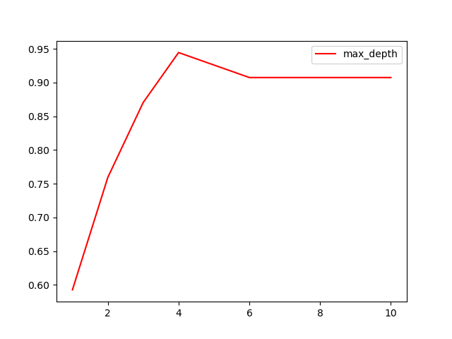
reflection:
- Can pruning parameters certainly improve the performance of the model in the test set? - there is no absolute answer to parameter tuning. Everything depends on the data itself.
- So many parameters, draw learning curves one by one? - in the case of Titanic, we will answer this question.
In any case, the default value of pruning parameters will make the trees grow endlessly. These trees may be very huge on some data sets and consume a lot of memory. Therefore, if you have a very large data set and you have predicted that you will prune anyway, it would be better to set these parameters in advance to control the complexity and size of the tree.
2.1.4 target weight parameters
[1]class_weight & min_weight_fraction_leaf
Parameters to complete sample label balance. Sample imbalance means that in a set of data sets, a class of labels naturally accounts for a large proportion. For example, in the bank, it is necessary to judge whether "a person with a credit card will default", that is, the proportion of yes vs no (1%: 99%). Under this classification condition, even if the model does nothing, it can predict the results as "no", and the accuracy can be 99%. So we want to make class_ The weight parameter balances the sample labels, gives more weight to a small number of labels, makes the model more inclined to a few classes, and models in the direction of capturing a few classes. This parameter defaults to None, and this mode indicates automatic feeding
The same weight as all labels in the dataset.
With the weight, the sample size is no longer simply the number of records, but is affected by the input weight. Therefore, pruning needs to be combined at this time_ weight_ fraction_ Leaf is used as a weight based pruning parameter. Also note that weight based pruning parameters (such as min_weight_fraction_leaf) will be less biased towards the dominant class than criteria that do not know the sample weight (such as min_samples_leaf). If the samples are weighted, it is easier to optimize the tree structure using the weight based pre pruning criteria, which ensures that the leaf nodes contain at least a small part of the sum of the sample weights.
2.2 important attributes and interfaces
Attributes are various properties of the model that can be called to view after model training. For the decision tree, the most important is the feature_importances_, Be able to view the importance of each feature to the model.
The interfaces of many algorithms in sklearn are similar. For example, fit and score, which we have used before, can be used for almost every algorithm. In addition to these two interfaces, the most commonly used interfaces for decision trees are apply and predict. The input test set in apply returns the index of the leaf node where each test sample is located, and the predict input test set returns the label of each test sample. The returned content is clear and very easy.
It must be mentioned here that x is required in all interfaces_ Train and X_test, the input characteristic matrix must be at least a two-dimensional matrix. sklearn does not accept any one-dimensional matrix as input of characteristic matrix. If your data does have only one feature, you must use reshape(-1,1) to add dimension to the matrix; If your data has only one feature and one sample, use reshape(1,-1) to add dimension to your data.
#apply returns the index of the leaf node where each test sample is located
clf.apply(Xtest)
#predict returns the classification / regression results of each test sample
clf.predict(Xtest)
Decision tree summary:
[1] Eight parameters: Criterion, two random_state, splitter, five pruning parameters (max_depth,min_samples_split, min_samples_leaf, max_feature, min_impulse_decrease)
[2] One attribute: feature_importances_
[3] Four interfaces: fit, score, apply, predict
3 .DecisionTreeRegressor
class sklearn.tree.DecisionTreeRegressor (criterion='mse',
					splitter='best',
					max_depth=None,
					min_samples_split=2,
					min_samples_leaf=1,
					min_weight_fraction_leaf=0.0,
					max_features=None,
					random_state=None,
					max_leaf_nodes=None,
					min_impurity_decrease=0.0,
					min_impurity_split=None,
					presort=False)
As like as two peas, almost all parameters, attributes and interfaces are exactly the same as classification trees. It should be noted that in the regression tree species, there is no question of whether the label distribution is balanced, so there is no class_ Parameters such as weight.
3.1 important parameters, attributes and interfaces
[1]criterion
Regression tree is an indicator of branch quality, and supports three standards:
(1) Enter "mse" to use the mean square error (mse). The difference between the mean square error between the parent node and the leaf node will be used as the criterion for feature selection. This method minimizes L2 loss by using the mean value of the leaf node
(2) Enter "friedman_mse" to use Feldman mean square error, which uses Friedman's improved mean square error for problems in potential branching
(3) Enter "MAE" to use the absolute mean error MAE (mean absolute error). This indicator uses the median value of leaf nodes to minimize L1 loss. The most important attribute is still feature_importances_, The interface is still the core of apply, fit, predict and score.

Where N is the number of samples, i is each data sample, fi is the value regressed by the model, and yi is the actual value label of sample point i. Therefore, the essence of MSE is actually the difference between the sample real data and the regression results. In the regression tree, MSE is not only our branch quality measurement index, but also our most commonly used index to measure the regression quality of the regression tree. When we use cross validation or other methods to obtain the results of the regression tree, we often choose the mean square error as our evaluation (in the classification tree, this index is the prediction accuracy represented by score). In regression, what we pursue is that the smaller the MSE, the better.
However, the regression tree interface score returns r square, not MSE. R squared is defined as follows:
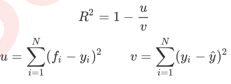
Where u is the sum of squares of residuals (MSE * N), v is the sum of squares, N is the number of samples, i is each data sample, fi is the value regressed by the model, and yi is the actual value label of sample point i. The y cap is the average number of real value labels. R squared can be positive or negative (if the sum of squared residuals of the model is much greater than
The sum of squares of the model. If the model is very bad, R square will be negative), and the mean square error will always be positive.
It is worth mentioning that although the mean square error is always positive, when the mean square error is used as the evaluation standard in sklearn, the "neg_mean_squared_error" is calculated . this is because when sklearn calculates the model evaluation index, it will consider the nature of the index itself. The mean square error itself is an error, so sklearn is divided into a loss of the model. Therefore, in sklearn, it is expressed as a negative number. The real mean square error MSE value is actually the number with the negative sign removed from neg_mean_squared_error.
Take a quick look at how regression trees work:
from sklearn.datasets import load_boston
from sklearn.model_selection import cross_val_score
from sklearn.tree import DecisionTreeRegressor
boston = load_boston()
regressor = DecisionTreeRegressor(random_state=0)
cross_val_score(regressor, boston.data, boston.target, cv=10,
        scoring = "neg_mean_squared_error")
#Cross validation cross_val_score usage
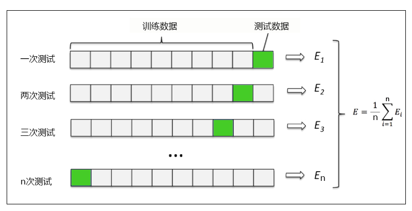
Cross validation is a method to observe the stability of the model. We divide the data into n parts, one of which is used as the test set and the other n-1 parts as the training set, and calculate the accuracy of the model for many times to evaluate the average accuracy of the model. The division of the training set and the test set will interfere with the results of the model, so
The average value obtained from the results of cross validation n times is a better measure of the effect of the model.
3.2 example: image rendering of one-dimensional regression
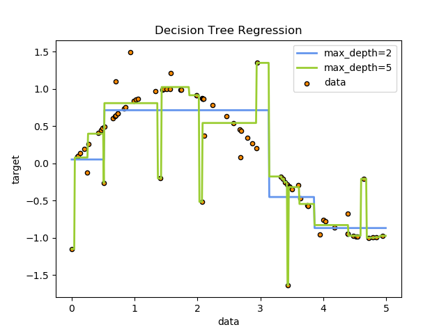
Next, we go to the two-dimensional plane to observe how the decision tree fits a curve. We use the regression tree to fit the sinusoidal curve and add some noise to observe the performance of the regression tree.
1. Import the required library
import numpy as np
from sklearn.tree import DecisionTreeRegressor
import matplotlib.pyplot as plt
2. Create a sinusoidal curve with noise
In this step, our basic idea is to create a group of random values (x) of abscissa axis distributed on 0 ~ 5, then put this group of values into sin function to generate the value (y) of ordinate, and then add noise to y. Throughout the process, we will use the numpy library to generate this sine curve for us.
rng = np.random.RandomState(1)
X = np.sort(5 * rng.rand(80,1), axis=0)
y = np.sin(X).ravel()
y[::5] += 3 * (0.5 - rng.rand(16))
#Np.random.rand (array structure), a function that generates random arrays
#Understand the usage of the dimensionality reduction function travel()
np.random.random((2,1))
np.random.random((2,1)).ravel()
np.random.random((2,1)).ravel().shape
3. Instantiation & Training Model
regr_1 = DecisionTreeRegressor(max_depth=2)
regr_2 = DecisionTreeRegressor(max_depth=5)
regr_1.fit(X, y)
regr_2.fit(X, y)
4. Import the test set into the model and predict the results
X_test = np.arange(0.0, 5.0, 0.01)[:, np.newaxis]
y_1 = regr_1.predict(X_test)
y_2 = regr_2.predict(X_test)
#Np.array (start point, end point, step size) function to generate an ordered array
#Understand the usage of dimension increasing slice np.newaxis
l = np.array([1,2,3,4])
print(l)
print(l.shape)
print(l[:,np.newaxis])
print(l[:,np.newaxis].shape)
print(l[np.newaxis,:].shape)
print("----"*30)
5. Draw image
plt.figure()
plt.scatter(X, y, s=20, edgecolor="black",c="darkorange", label="data")
plt.plot(X_test, y_1, color="cornflowerblue",label="max_depth=2", linewidth=2)
plt.plot(X_test, y_2, color="yellowgreen", label="max_depth=5", linewidth=2)
plt.xlabel("data")
plt.ylabel("target")
plt.title("Decision Tree Regression")
plt.legend()
plt.show()

It can be seen that the regression tree learns the local linear regression of approximate sinusoidal curve. We can see that if the maximum depth of the tree (controlled by the max_depth parameter) is set too high, the decision tree learns too fine. It learns a lot of details from the training data, including the presentation of noise, so that the model deviates from the real sinusoidal curve and forms over fitting.
4. Example: prediction of Titanic survivors
The sinking of the Titanic is one of the most serious maritime accidents in the world. Today, we use the classification tree model to predict who may become survivors.
Dataset from https://www.kaggle.com/c/titanic . The data set contains two csv format files. Data is the data we will use next, and test is the test set provided by kaggle.
1. Import the required library
import pandas as pd
from sklearn.tree import DecisionTreeClassifier
from sklearn.model_selection import train_test_split
from sklearn.model_selection import GridSearchCV
from sklearn.model_selection import cross_val_score
import matplotlib.pyplot as plt
2. Import datasets and explore data
data = pd.read_csv(r"data.csv",index_col= 0)
print(data.head())
print(data.info())
3. Preprocess the data set
#Delete columns with too many missing values and columns that have nothing to do with the predicted y according to observation and judgment
data.drop(["Cabin","Name","Ticket"],inplace=True,axis=1)
#Deal with missing values and fill in columns with more missing values. Some features only confirm one or two values. You can directly delete records
data["Age"] = data["Age"].fillna(data["Age"].mean())
data = data.dropna()
#Convert classified variables to numeric variables
#Convert binary variables to numeric variables
#Astype can convert a pandas object to a certain type. Unlike apply(int(x)), astype can convert text classes to numbers. In this way, it is easy to convert binary classification features to 0 ~ 1
data["Sex"] = (data["Sex"]== "male").astype("int")
#Convert three category variables to numeric variables
labels = data["Embarked"].unique().tolist()
data["Embarked"] = data["Embarked"].apply(lambda x: labels.index(x))
#View processed dataset
print(data.head())
4. Extract the label and feature matrix, which is divided into test set and training set
X = data.iloc[:,data.columns != "Survived"]
y = data.iloc[:,data.columns == "Survived"]
from sklearn.model_selection import train_test_split
Xtrain, Xtest, Ytrain, Ytest = train_test_split(X,y,test_size=0.3)
#Fix the index of test set and training set
for i in [Xtrain, Xtest, Ytrain, Ytest]:
	i.index = range(i.shape[0])

#View divided training sets and test sets
Xtrain.head()
5. Import the model and check the results roughly
clf = DecisionTreeClassifier(random_state=25)
clf = clf.fit(Xtrain, Ytrain)
score_ = clf.score(Xtest, Ytest)
score_
score = cross_val_score(clf,X,y,cv=10).mean()
score
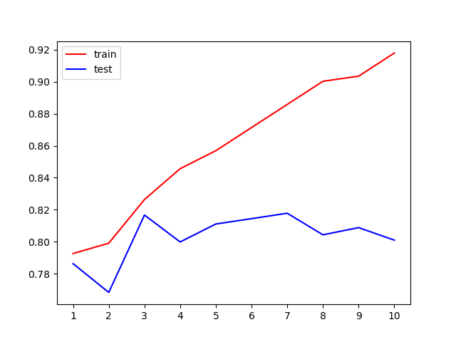
6. Under different conditions_ Observe the fitting condition of the model under depth
tr = []
te = []
for i in range(10):
    clf = DecisionTreeClassifier(random_state=25
        ,max_depth=i+1
        ,criterion="entropy"
        )
    clf = clf.fit(Xtrain, Ytrain)
    score_tr = clf.score(Xtrain,Ytrain)
    score_te = cross_val_score(clf,X,y,cv=10).mean()
    tr.append(score_tr)
    te.append(score_te)

print(max(te))
plt.plot(range(1,11),tr,color="red",label="train")
plt.plot(range(1,11),te,color="blue",label="test")
plt.xticks(range(1,11))
plt.legend()
plt.show()
#Why use "entry" here? We notice that when the maximum depth is 3, the model fitting is insufficient, and the performance in the training set and the test set is close, but it is not very ideal, which can only reach about 83%, so we need to use entropy.
7. Use grid search to adjust parameters
import numpy as np
gini_thresholds = np.linspace(0,0.5,20)
parameters = {'splitter':('best','random')
                ,'criterion':("gini","entropy")
                ,"max_depth":[*range(1,10)]
                ,'min_samples_leaf':[*range(1,50,5)]
                ,'min_impurity_decrease':[*np.linspace(0,0.5,20)]
                }
clf = DecisionTreeClassifier(random_state=25)
GS = GridSearchCV(clf, parameters, cv=10)
GS.fit(Xtrain,Ytrain)
print(GS.best_params_)
print(GS.best_score_)
5. Advantages and disadvantages of decision tree
Advantages of decision tree
1. Easy to understand and explain, because trees can be painted and seen
2. Little data preparation is required. Many other algorithms usually need data normalization, creating virtual variables and deleting null values. But please note,
sklearn The decision tree module in does not support the processing of missing values.
3. The cost of using the tree (for example, when predicting data) is the logarithm of the number of data points used to train the tree. Compared with other algorithms, this is
 A very low cost.
4. It can process digital and classified data at the same time, and can do both regression and classification. Other techniques are usually dedicated to analyzing classes with only one variable
 Type data set.
5. Be able to handle multiple output problems, that is, problems with multiple labels. Pay attention to distinguish them from problems with multiple label classifications in one label
6. It is a white box model, and the results can be easily explained. If a given situation can be observed in the model, it can be easily realized by Boolean logic
 Explain the conditions. On the contrary, in the black box model (for example, in artificial neural networks), the results may be more difficult to explain.
7. Statistical tests can be used to validate the model, which allows us to consider the reliability of the model.
8. Even if its assumptions violate the real model of generated data to some extent, it can perform well.
Disadvantages of decision tree
1. Decision tree learners may create too complex trees, which can not promote the data well. This is called overfitting. Trim, set leaf nodes
 The minimum number of samples required or the maximum depth of the tree are necessary to avoid this problem, and the integration and adjustment of these parameters is very important for beginners
 It will be more obscure
2. The decision tree may be unstable, and small changes in the data may lead to the generation of completely different trees. This problem needs to be solved by integration algorithm.
3. The learning of decision tree is based on greedy algorithm, which tries to achieve the overall optimization by optimizing the local optimization (the optimization of each node)
It is not guaranteed to return the global optimal decision tree. This problem can also be solved by integration algorithm. In random forest, features and samples will branch
 It is randomly sampled in the process.
4. Some concepts are difficult to learn because decision trees are not easy to express, such as XOR,Parity or multiplexer problems.
5. If some classes in the tag are dominant, the decision tree learner will create a tree biased towards the dominant class. Therefore, it is recommended to balance before fitting the decision tree
 Data set.