1. Logistic Regression

1.1 Logistic Regression & Perceptron

1.2 definition of logistic regression model

1.3 maximum likelihood estimation model parameters

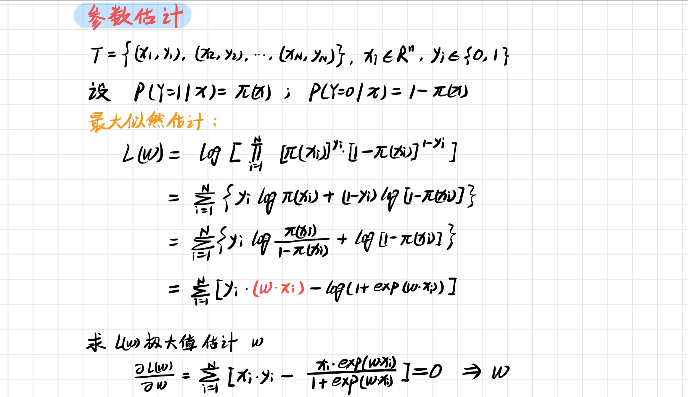
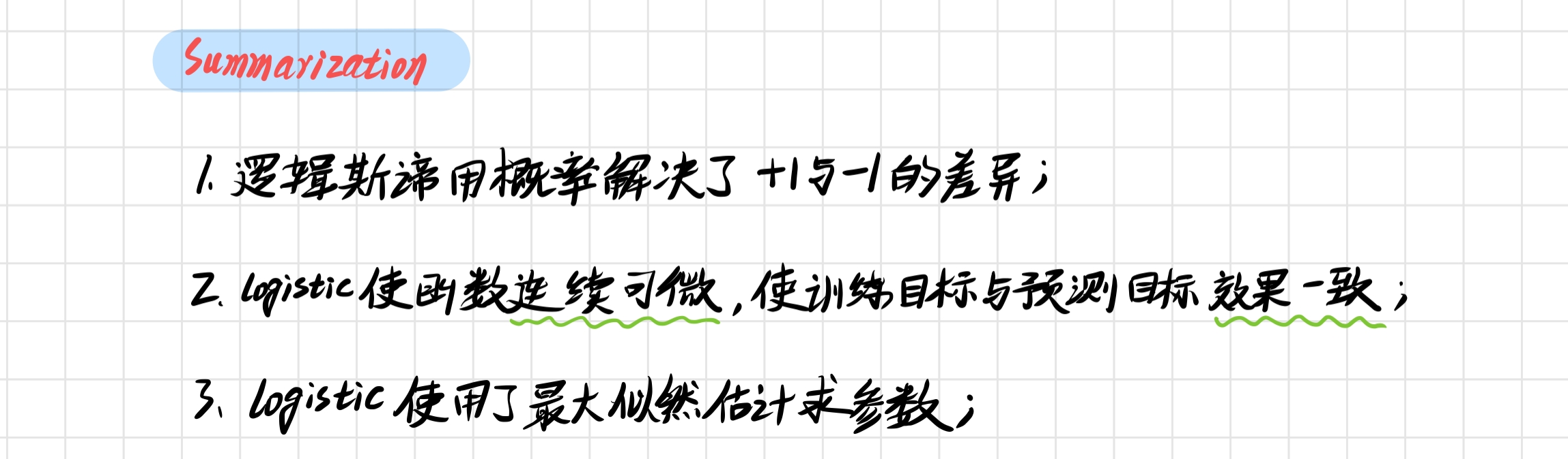
summary

2. Python implementation of logistic regression

2.1 data sets

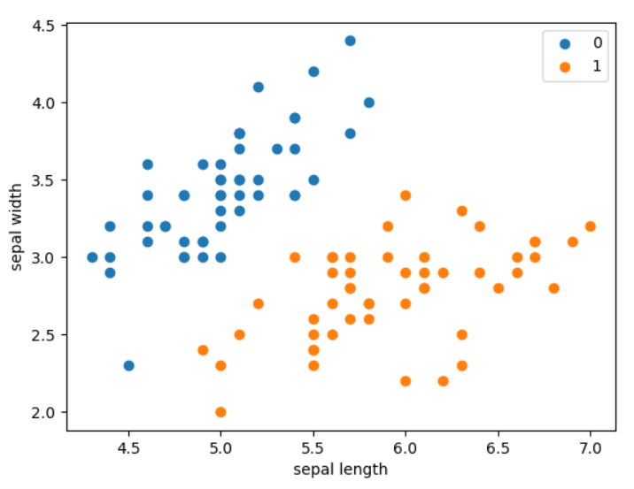
The data set is Iris data set, which contains two types of flowers. Each sample contains two characteristics and one category. Set the ratio of test set to training set as 1:4:

from math import exp
import numpy as np
import pandas as pd
import matplotlib.pyplot as plt
from sklearn.datasets import load_iris
from sklearn.model_selection import train_test_split

def create_data():
    iris = load_iris()
    df = pd.DataFrame(data=iris.data, columns=iris.feature_names)
    df['label'] = iris.target
    df.columns = ['sl', 'sw', 'pl', 'pw', 'label']
    data = np.array(df.iloc[:100, [0, 1, -1]])
    return data[:, [0, 1]], data[:, -1]

X, y = create_data()
X_train, X_test, y_train, y_test = train_test_split(X, y, test_size=0.2)

plt.scatter(X[:50, 0], X[:50, 1], label='0')
plt.scatter(X[50:, 0], X[50:, 1], label='1')
plt.xlabel('sepal length')
plt.ylabel('sepal width')
plt.legend()
plt.show()

The results are as follows:

2.2 building models

Next, we build the model of LogisticRegressionClassifier:

class LogisticRegressionClassifier:
	# Maximum number of iterations and learning step
    def __init__(self, max_iter=200, learning_rate=0.01):
        self.max_iter = max_iter
        self.learning_rate = learning_rate

    def sigmoid(self, x):
        return 1 / (1 + exp(-x))

    def expand(self, X):
        matrix = []
        for item in X:
            matrix.append([*item, 1.0])
        return matrix

    def fit(self, X, y):
        X = self.expand(X)
        self.weights = np.zeros((len(X[0]), 1), dtype=np.float32) # columnn matrice

        for iter_ in range(self.max_iter):
            for item_x, item_y in zip(X, y):
                res = self.sigmoid(np.dot(item_x, self.weights))
                self.weights += self.learning_rate * (item_y - res) * np.transpose([item_x]) 
        print(f'LogisticRegression Model(learning_rate={self.learning_rate}, max_iter={self.max_iter}')

    def score(self, X_test, y_test):
        success = 0
        expanded_X = self.expand(X_test)
        for X, y in zip(expanded_X, y_test):
            predict_res = np.dot(X, self.weights) > 0.5
            if predict_res == y:
                success += 1
        return success / len(X_test)

explain

(1) Note that the sigmoid function uses exp(-x), because using exp(x) may overflow!

(2) The expand function extends X by adding a 1

(3) The fitting function fit() is similar to the perceptron. Its principle is to calculate the parameters by maximum likelihood estimation. The maximum value can be calculated by random gradient. The principle is as follows:

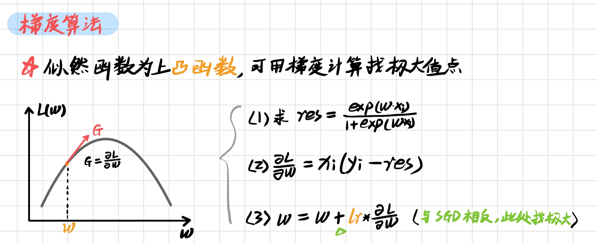
The corresponding code is:

for x, y in zip(X, y) can get X and Y corresponding to the index one by one;

np. The transfer function can transpose the matrix, NP Dot () can perform matrix multiplication;

def fit(self, X, y):
    X = self.expand(X)
    self.weights = np.zeros((len(X[0]), 1), dtype=np.float32) # columnn matrice

    for iter_ in range(self.max_iter):
        for item_x, item_y in zip(X, y):
            res = self.sigmoid(np.dot(item_x, self.weights))
            self.weights += self.learning_rate * (item_y - res) * np.transpose([item_x]) 

(4) During prediction, judge whether sigmoid(wx) is greater than 0.5, less than 0.5, and it is judged as 0 or 1

2.3 test results

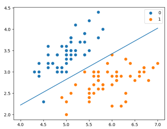
Let's test the score of the model:

clf = LogisticRegressionClassifier()
clf.fit(X_train, y_train)
print(clf.score(X_test, y_test))

x_ponits = np.arange(4, 8)
y_ = -(clf.weights[0]*x_ponits + clf.weights[2])/clf.weights[1]
plt.plot(x_ponits, y_)
plt.scatter(X[:50,0],X[:50,1], label='0')
plt.scatter(X[50:,0],X[50:,1], label='1')
plt.legend()
plt.show()

Prediction score 1.0 🍻

3. Scikit learn instance

3.1 LogisticRegression

stay scikit-learn The Linear Model contains the model LogisticRegression , the use method can refer to sklearn.linear_model.LogisticRegression¶:

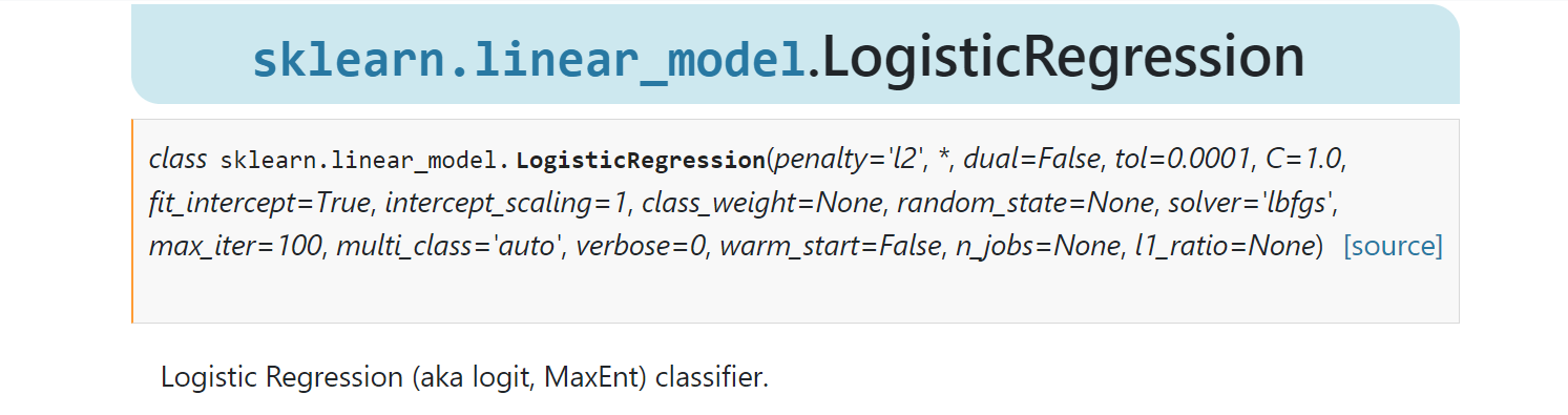
Parameter solver

solver parameter determines our optimization method for logistic regression loss function. There are four algorithms to choose from, namely:

• a) liblinear: it is implemented using the open source liblinear library and internally uses the coordinate axis descent method to iteratively optimize the loss function.
• b) lbfgs: a kind of quasi Newton method, which uses the second derivative matrix of loss function, i.e. Hessian matrix, to iteratively optimize the loss function.
• c) Newton CG: it is also a kind of Newton method family. It uses the second derivative matrix of loss function, i.e. Hessian matrix, to iteratively optimize the loss function.
• d) sag: random average gradient descent, which is a variant of the gradient descent method. The difference from the ordinary gradient descent method is that only a part of the samples are used to calculate the gradient in each iteration, which is suitable for the case of large sample data.

3.2 Example

import numpy as np
import pandas as pd
from sklearn.datasets import load_iris
from sklearn.model_selection import train_test_split
from sklearn.linear_model import LogisticRegression

def create_data():
    iris = load_iris()
    df = pd.DataFrame(data=iris.data, columns=iris.feature_names)
    df['label'] = iris.target
    df.columns = ['sl', 'sw', 'pl', 'pw', 'label']
    data = np.array(df.iloc[:100, [0, 1, -1]])
    return data[:, [0, 1]], data[:, -1]

X, y = create_data()
X_train, X_test, y_train, y_test = train_test_split(X, y, test_size=0.2)

clf = LogisticRegression(max_iter=200)
clf.fit(X_train, y_train)
print(clf.score(X_test, y_test))
print(clf.coef_, clf.intercept_)

give the result as follows

1.0
[[ 2.86401035 -2.76369768]] [-6.92179114]

The first item in the last line is w, and the last is a separate part b

REFERENCE

1. Li Hang's statistical learning method
2. machine learning
3. scikit-learn