1. Theoretical part

1.1 K nearest neighbor method

1． k k k-nearest neighbor method is a basic and simple classification and regression method. k k The basic method of k-nearest neighbor method is: for a given training instance point and input instance point, first determine the value of input instance point k k k nearest neighbor training instance points, and then use this k k The number of classes of k training instance points is used to predict the class of input instance points.

2． k k The k-nearest neighbor model corresponds to a partition of the feature space based on the training data set. k k In the k-nearest neighbor method, when the training set, distance measurement k k After the k value and classification decision rules are determined, the result is uniquely determined.

3． k k Three elements of k-nearest neighbor method: distance measurement k k k-value selection and classification decision rules. The commonly used distance measures are Euclidean distance and more general distance L p L_p Lp = distance. k k k value hours, k k k-nearest neighbor model is more complex; k k When the value of k is large, k k k-nearest neighbor model is simpler. k k The choice of k value reflects the trade-off between approximation error and estimation error, and the optimal one is usually selected by cross validation k k k.

The common classification decision rule is majority voting, which corresponds to empirical risk minimization.

4． k k The implementation of k-nearest neighbor method needs to consider how to quickly search k nearest neighbors. kd tree is a kind of data structure which is convenient for fast retrieval of data in k-dimensional space. The kd tree is a binary tree that represents a pair of k k A partition of k-dimensional space in which each node corresponds to k k A super rectangular region in k-dimensional space partition. Using kd tree can save the search of most data points, so as to reduce the amount of calculation.

1.2 distance measurement

Set feature space x x x is n n n-dimensional real vector space x i , x j ∈ X x_{i}, x_{j} \in \mathcal{X} xi​,xj​∈X

x i = ( x i ( 1 ) , x i ( 2 ) , ⋯   , x i ( n ) ) T x_{i}=\left(x_{i}^{(1)}, x_{i}^{(2)}, \cdots, x_{i}^{(n)}\right)^{\mathrm{T}} xi​=(xi(1)​,xi(2)​,⋯,xi(n)​)T
x j = ( x j ( 1 ) , x j ( 2 ) , ⋯   , x j ( n ) ) T x_{j}=\left(x_{j}^{(1)}, x_{j}^{(2)}, \cdots, x_{j}^{(n)}\right)^{\mathrm{T}} xj​=(xj(1)​,xj(2)​,⋯,xj(n)​)T

be x i x_i xi​, x j x_j xj + L p L_p Lp} distance is defined as:

L p ( x i , x j ) = ( ∑ i = 1 n ∣ x i ( i ) − x j ( l ) ∣ p ) 1 p L_{p}\left(x_{i}, x_{j}\right)=\left(\sum_{i=1}^{n}\left|x_{i}^{(i)}-x_{j}^{(l)}\right|^{p}\right)^{\frac{1}{p}} Lp​(xi​,xj​)=(∑i=1n​∣∣∣​xi(i)​−xj(l)​∣∣∣​p)p1​

• p = 1 p= 1 p=1 Manhattan distance
• p = 2 p= 2 p=2 Euclidean distance
• p = ∞ p= \infty p = ∞ Chebyshev distance

Python code implementation:

import math

def L(x, y, p=2):
	sum = 0
	for i in range(len(x)):
		sum += math.pow(abs(x[i] - y[i]), p)
	return math.pow(sum, 1/p)

2. Python implementation of k-nearest neighbor method

2.1 data set preprocessing

For convenience, we used Iris Dataset:

import numpy as np
import pandas as pd
import matplotlib.pyplot as plt
from sklearn.datasets import load_iris
from collections import Counter
from sklearn.model_selection import train_test_split

iris = load_iris()
df = pd.DataFrame(data=iris.data, columns=iris.feature_names)
df['label'] = iris.target
df.columns = ['sepal length', 'sepal width', 'petal length', 'petal width', 'label']

data = np.array(df.iloc[:100, [0, 1, -1]])
X, y = data[:, :-1], data[:, -1]
X_train, X_test, y_train, y_test = train_test_split(X, y, test_size=0.2)
print(f'data.shape: {data.shape}')
print(f'X_train.shape: {X_train.shape}')
print(f'X_test.shape: {X_test.shape}')
print(f'y_train.shape: {y_train.shape}')
print(f'y_test.shape: {y_test.shape}')

We used the first 100 rows of data, including 2 types of flowers, 50 samples in each type, and each sample has 4 eigenvalues

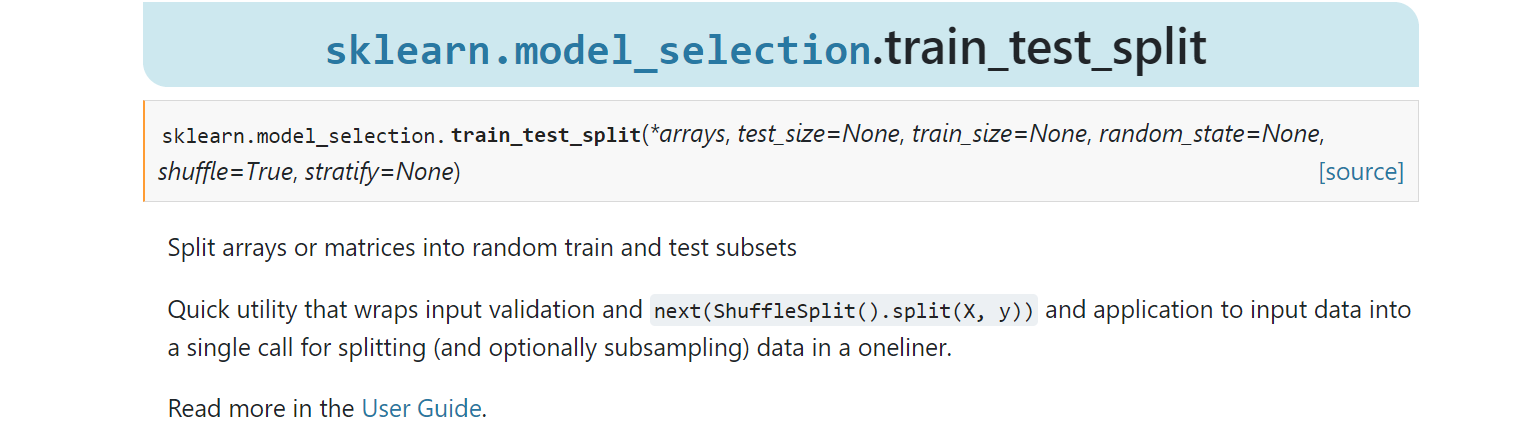
Then we used sklearn model_ Train of selection module_ test_ Split method divides the data set into training data and test data, of which 20% is test data. For specific usage methods, refer to: sklearn.model_selection.train_test_split

The output results are as follows:

data.shape: (100, 3)
X_train.shape: (80, 2)
X_test.shape: (20, 2)
y_train.shape: (80,)
y_test.shape: (20,)

2.2 model construction

The model includes three methods: initialization construction KNN(), prediction (x) and prediction accuracy score(X_test, y_test):

from functools import cmp_to_key

class KNN:
	def __init__(self, X_train, y_train, n_neighbors=3, p=2):
		self.n = n_neighbors
		self.p = p
		self.X_train = X_train
		self.y_train = y_train

	def predict(self, X):
		# n nearest neighbors
		knn_list = []
		# distance from X to all neighbors
		distances = [L(X, point, self.p) for point in X_train]
		# sort by distance
		items = list(zip(X_train, y_train, distances))
		items.sort(key=cmp_to_key(lambda item1, item2: item1[-1]-item2[-1]))

		# decide
		knn_list = [item[0] for item in items[:self.n]]
		class_list = [item[1] for item in items[:self.n]]
		c = Counter(class_list).most_common()
		return Counter(class_list).most_common()[0][0]

	def score(self, X_test, y_test):
		right_count = 0
		for X, y in zip(X_test, y_test):
			if self.predict(X) == y:
				right_count += 1
			else:
				print(X, y)
		return right_count / len(X_test)

The Counter() container, zip() method and list are used sort() sort , for example:

from collections import Counter
from functools import cmp_to_key

L = list('eabcdabcaba')
c = Counter(L)
print(c)
print(c.most_common())

words = [item[0] for item in c.most_common()]
freqc = [item[1] for item in c.most_common()]
print(words, freqc)

items = list(zip(words, freqc))
print(items)

items.sort(key=cmp_to_key(lambda x, y: x[1] - y[1]))
print(items)

The result is:

Counter({'a': 4, 'b': 3, 'c': 2, 'e': 1, 'd': 1})
[('a', 4), ('b', 3), ('c', 2), ('e', 1), ('d', 1)]
['a', 'b', 'c', 'e', 'd']
[4, 3, 2, 1, 1]

2.3 test model

Use the remaining 20% of the data for testing:

clf = KNN(X_train, y_train)
score = clf.score(X_test, y_test)
print(score)	# 1.0

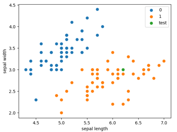
print(clf.predict([6.2, 3]))	# 1.0
plt.scatter(df[:50]['sepal length'], df[:50]['sepal width'], label='0')
plt.scatter(df[50:100]['sepal length'], df[50:100]['sepal width'], label='1')
plt.scatter(6.2, 3, label='test')
plt.xlabel('sepal length')
plt.ylabel('sepal width')
plt.legend()
plt.show()

The prediction success rate reached 100% 🍻

Draw space division:

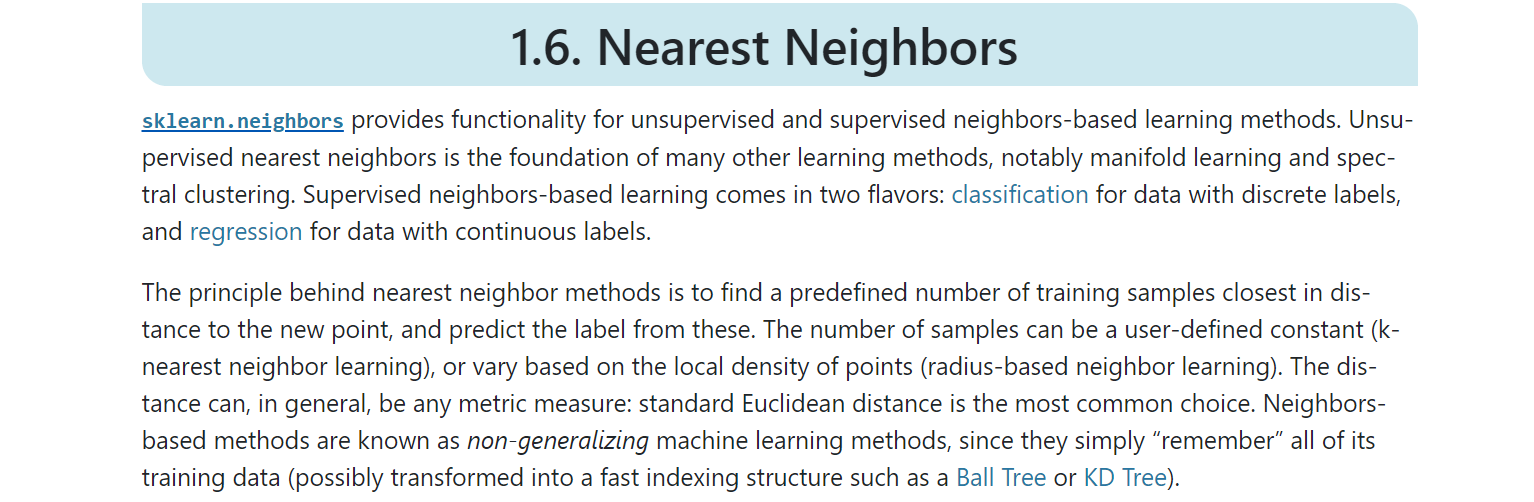
2.4 scikit-learn

sklearn.neighbors The nearest neighbor algorithm is defined. What we need to use is sklearn.neighbors.KNeighborsClassifier Classifier:

from sklearn.neighbors import KNeighborsClassifier

clf = KNeighborsClassifier(n_neighbors=3, p=2)
clf.fit(X_train, y_train)
score = clf.score(X_test, y_test)
print(f'score = {score}')	# 1.0

The main parameters of kneigborsclassifier () are as follows (refer to the official website):

• n_neighbors: number of adjacent points
• p: Distance measurement
• Algorithm: nearest neighbor algorithm, optional {'auto', 'ball_tree', 'kd_tree', 'brute'}
• weights: determines the weight of the nearest neighbor

3. kd tree

kd tree is a kind of tree data structure that stores instance points in k-dimensional space for fast retrieval. kd tree is a binary tree that represents a partition of a dimensional space. Constructing kd tree is equivalent to continuously dividing the 𝑘 dimensional space with a hyperplane perpendicular to the coordinate axis to form a series of k-dimensional hyper rectangular regions. Each node of kd tree corresponds to a hyper rectangular region.

3.1 algorithm for constructing balanced kd tree

Input: k k k-dimensional spatial dataset T ＝ x 1 , x 2 , ... , x N T＝{x_1, x_2,...,x_N} T＝x1​,x2​,...,xN​，

among x i = ( x i ( 1 ) , 𝑥 i ( 2 ) , ⋯ , x i ( k ) ) T , i ＝ 1 , 2 , ... , N x_i=(x_{i}^{(1)},𝑥_i^{(2)},⋯,x_i^{(k)})^T, i＝1,2,...,N xi​=(xi(1)​,xi(2)​,⋯,xi(k)​)T,i＝1,2,...,N；

Output: kd tree

start

• Construct the root node, which corresponds to the containing T T T k k Hyperrectangular region of k-dimensional space.
• choice x ( 1 ) x^{(1)} x(1) is the coordinate axis, taking the coordinates of all instances in T x ( 1 ) x^{(1)} The median of x(1) coordinate is the tangent point, and the super rectangular region corresponding to the root node is divided into two sub regions. Syncopation consists of passing through the syncopation point and with the coordinate axis x ( 1 ) x^{(1)} x(1) vertical hyperplane implementation.
• Generate left and right child nodes with a depth of 1 from the root node: the corresponding coordinates of the left child node x ( 1 ) x^{(1)} x(1) is smaller than the sub region of the tangent point, and the right sub node corresponds to the coordinate x ( 1 ) x^{(1)} x(1) is greater than the sub region of the tangent point.
• Save the instance points falling on the tangent hyperplane at the root node.

repeat

• For depth j j j node, select x ( l ) x^{(l)} x(l) is the tangent coordinate axis, l ＝ j ( m o d k ) + 1 l＝j(modk)+1 l = j(modk)+1, based on the number of all instances in the region of the node x ( l ) x^{(l)} The median of x(l) coordinate is the tangent point, and the hyperrectangular region corresponding to the node is divided into two sub regions. Syncopation consists of passing through the syncopation point and with the coordinate axis x ( l ) x^{(l)} x(l) vertical hyperplane implementation.
• The depth generated by this node is j + 1 j+1 Left and right child nodes of j+1: the corresponding coordinates of the left child node x ( l ) x^{(l)} x(l) is smaller than the sub region of the tangent point, and the corresponding coordinates of the right sub node x ( l ) x^{(l)} x(l) is greater than the sub region of the tangent point.
• Save the instance points falling on the tangent hyperplane at this node.

end

• Stop until no instances of the two sub regions exist. So as to form the region division of kd tree.

3.2 Python implementation of KD tree

kd tree node

Each node stores the dimensions of the current spatial division. The elements of the node, the left child node and the right child node:

class Node:
	def __init__(self, elem, split, left, right):
		self.elem = elem
		self.split = split	# dimension-id
		self.left = left
		self.right = right

Constructing kd tree

First, record the total number of dimensions divided by space, and then recursively start from the root node and recurse to the left and right child nodes:

Each node stores the "Midpoint" under the current space division conditions. For each sequence with division, first sort it according to the division dimension, take out the median and put it into the node, and put the remaining sequences into the left child node and the right child node for recursion (the dimension of space division increases automatically. Split = (split + 1)% k)

class KdTree:
	def __init__(self, data):
		k = len(data[0])	# dimentions

		def createNode(split, data_set):
			if not data_set:
				return None
			data_set.sort(key=lambda x: x[split])
			split_pos = len(data_set) // 2
			median = data_set[split_pos]
			split_next = (split + 1) % k
			return Node(
				median,
				split,
				createNode(split_next, data_set[:split_pos]),
				createNode(split_next, data_set[split_pos+1:]))

		self.root = createNode(0, data)

Next, we create a kd tree and traverse the hierarchy to see the results:

def levelorder(root):
	queue = []
	queue.append(root)
	while queue != []:
		curr = queue.pop(0)
		if curr.left:
			queue.append(curr.left)
		if curr.right:
			queue.append(curr.right)
		print(curr.elem)

L = [[2, 3], [5, 4], [9, 6], [4, 7], [8, 1], [7, 2]]
tree = KdTree(L)
levelorder(tree.root)

The results are as follows:

[7, 2]
[5, 4]
[9, 6]
[2, 3]
[4, 7]
[8, 1]

forecast

Use kd tree to find the nearest point:

• First, look down from the root node. If the value of the current partition dimension is less than the value of the node, look to the left, otherwise look to the right until you reach the root node, and treat this point as a nearest
• Back up from the current leaf node. If the node is closer to the target, update the nearest; Find out whether another child node of the current nearest neighbor node has a closer point (detect whether the region division of the other child node intersects with the sphere composed of the distance between the target point and the nearest) and, if so, jump to another node to find the nearest neighbor; If not, continue to retreat upward;
• Repeat the previous step until you reach the root node and return to nearest

REFERENCES:

1. Li Hang's statistical learning method
2. scikit-learn
3. Introduction to Machine Learning with Python
4. lihang-code-master