scenario analysis

• Suppose the price of article a is 20.22 yuan / kg in 2000, 20.32 yuan / kg in 2001 and 21.01 yuan / kg in 2002. The middle price is omitted. Please predict the price of article a in 2022?
• This is a very simple linear regression case. We all know that we can predict the price in 2022 by drawing a straight line. So how to find this straight line?

Important concepts

• Cost function
• gradient descent

Cost function

• The more accurate we can draw a straight line on both sides, the more we can predict the cost
• The cost of each point and line is that when the value of x is the same, the y value corresponding to the point minus the square of the y value corresponding to the line becomes the symbolic representation ( y − h ) 2 (y - h) ^ 2 (y−h)2
• The cost function is to find an average cost. Considering that the derivative is required in the gradient descent method, in order to eliminate the multiplication of 2, the original function needs to be divided by 2. Therefore, the final expression of the cost function is J = 1 2 m Σ ( y − h ) 2 J = \frac{1}{2m}\Sigma(y - h) ^ 2 J=2m1​ Σ (y − h)2, where m is the number of samples
• What we want is to make this J J J min

gradient descent

• The gradient descent method is used to solve the problem of J J What is gradient descent for the problem of minimum J?
• Suppose a quadratic function of one variable is given y = x 2 y = x ^2 y=x2, q y y When y was the smallest, x x The value of x must be in x = 0 x = 0 When x=0, but the machine doesn't know x = 0 x = 0 When x=0, unless the solution formula is given, but generally there is no solution formula. At this time, it is necessary to derive the function to obtain the so-called extreme point. This time may be the minimum time.
• The gradient descent law takes advantage of the characteristics of the gradient and takes a random value at the beginning x x x. Then subtract a learning rate times the value of the derivative at this time, that is x − l r ∗ 2 x x - lr * 2x X − lr * 2x can always be infinitely close to x = 0 x = 0 x=0, although the final result may be x = 0.000001 x = 0.000001 x=0.000001, but it's enough for us
• For the cost function, the gradient descent method is also applicable, from which one can be obtained J J When the value of J is infinitely close to the minimum w w w， w w w is the weight of the line, because we already know x x The value range of x, so only the value of straight line is required k k k and b b b that's all

make a concrete analysis

• From the above two concepts, in order to get the straight line we want, we only need to initialize one b b b. One k k k. Then the gradient descent method is used b b b and k k k just keep updating, that is
  b = b − l r ∗ 1 m Σ ( h − y ) k = k − l r ∗ 1 m Σ ( h − y ) ∗ x i b = b - lr * \frac{1}{m}\Sigma(h - y)\\ k = k - lr * \frac{1}{m}\Sigma(h - y) * x_{i} b=b−lr∗m1​Σ(h−y)k=k−lr∗m1​Σ(h−y)∗xi​
• Why are the above two formulas different J J J seeking b b b and k k The partial derivative of k is this result

Implementation of univariate linear regression with custom python code

import matplotlib.pyplot as plt

# Cost function
def lose_function(b, k, x_data, y_data):
    '''
    Request price must be passed in b，k，x_data，y_data
    '''
    # For the cost, the final division of 2 is designed for 1/2m
    total_error = 0
    # m is the number of samples
    m = len(x_data)
    for i in range(m):
        total_error += (y_data[i] - (k * x_data[i] + b)) ** 2
    return total_error / m / 2

# Gradient descent function
def gradient_descent(b, k, x_data, y_data, epochs, lr):
    # m is the number of samples
    m = len(x_data)
    # epochs is the number of iterations
    for i in range(epochs):
        b_grad = 0
        k_grad = 0
        for j in range(len(x_data)):
            b_grad += (k * x_data[j] + b - y_data[j]) / m
            k_grad += (k * x_data[j] + b - y_data[j]) * x_data[j] / m
        b = b - lr * b_grad
        k = k - lr * k_grad
        # Record the number of iterations and the cost at this time
        print("The first{0}Iterations, lose={1}".format(i+1, lose_function(b, k, x_data, y_data)))
    return b, k

if __name__ == '__main__':
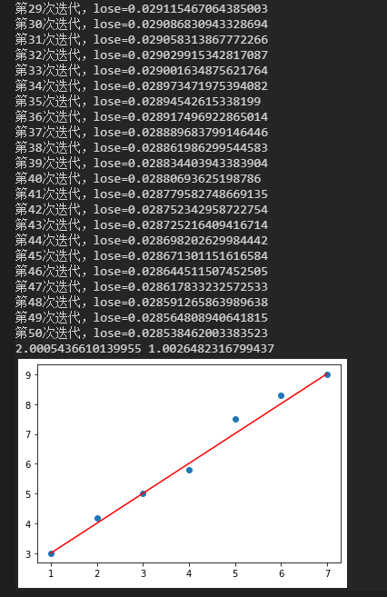
    x_data = [1, 2, 3, 4, 5, 6, 7]
    y_data = [3, 4.2, 5, 5.8, 7.5, 8.3, 9]
    plt.figure()
    plt.scatter(x_data, y_data)
    # Set the initial values of b and k
    k = 1
    b = 2
    # A smaller cost is obtained by iterative updating through the gradient descent method
    b, k = gradient_descent(b, k, x_data, y_data, 50, 0.0001)
    print(b, k)
    # After getting b and k, draw the fitting line
    plt.plot(x_data, [k * x + b for x in x_data], c='red')
    plt.show()

• The screenshot of the operation result is as follows