Deep learning and pytorch Foundation
Machine learning is a means to realize artificial intelligence. Its purpose is to enable programs to use past experience to learn independently and optimize answers
Deep learning is a specific method to realize machine learning
Model classification of machine learning
A specific problem can be solved through model - > Strategy - > algorithm
For data classification, we can divide the model into supervised learning model and unsupervised learning model
Supervised learning
As the name suggests, supervised learning is based on artificial marker supervision. In the data, through the data learning marker interface, we can use the decision function to achieve the purpose of prediction and analysis
Unsupervised learning
Because unsupervised learning does not mark the data, it has only different distribution for the data, and it can only produce the function of describing the data from the data distribution
Semi supervised learning
Semi supervised learning marks some data, which can reduce human work
Reinforcement learning
Reinforcement learning is like an upgrade of unsupervised learning, which is based on the results of unsupervised learning
parameter model
Based on the assumption of data distribution, the probability distribution function can be derived from sufficient data
Nonparametric model
The data itself has statistical characteristics, non parametric model adaptive data, and there are no specific data distribution parameters
Generation model
The generation model is to take the data of the supervised learning model as the object and use the joint distribution probability P ( X , Y ) P(X,Y) P(X,Y) modeling to generate function results corresponding to data
Discriminant model
The discriminant model is to predict the data results when the function is known
In the past, machine learning required a large amount of data and manual feedback results, resulting in the time-consuming and limited results of machine learning. Now we hope to use as little data as possible to give to machines for autonomous learning. However, machine learning is highly dependent on data, so there are still some problems, such as easy to be attacked by noise pollution, lack of associative reasoning ability, easy to be affected by extreme data, difficult to determine errors and so on.
Fundamentals of neural network
Inspired by the characteristics of neurons, such as multiple input and single output, asynchronous time and space, people use mathematical language to describe a function method, which is called activation function
Single layer perceptron
Activation function is equivalent to a processing function. When a function is activated under what conditions, it is analogous to what kind of output it can have under what kind of input. For different outputs, we can artificially define the special meaning corresponding to these output symbols. The nonlinear activation function can help us deal with more cases of data.
Due to the functional limitations of a single activation function, it can only turn a logical space into a limited part, and the classification operation has limitations, but the single-layer perceptron can not solve the nonlinear problem. In the logical space, because the activation function is equivalent to a line in the logical space, all the problems of nonlinear space division (i.e. the division of multiple lines) urgently need to be realized by multi-layer perceptron. Some columns of complex logic similar to digital logic can be realized by the logical combination of and or not gates. Using activation function, people have built a bridge from logical mathematics to digital mathematics.
Universal approximation theorem
If a hidden layer contains enough neurons, the three-layer feedforward neural network can approach any predetermined continuous function with any accuracy
The universal approximation theorem enlightens us that we can model any complex problem using neural network
The role of each layer of neural network
Mathematical formula of each layer y → = a ( W ⋅ x → + b ) \overrightarrow{y}=a(W·\overrightarrow{x}+b) y =a(W⋅x +b)
The spatial interpretation of linear algebra can be regarded as a series of spatial transformations of matrix space. Multiplying by a matrix is the distorted transformation of space, and the constant can be regarded as the translation of space
For the number of layers similar to the neural network, that is, increasing the number of activation functions, the activation function is a nonlinear function, that is, there are more regions in the space
The node can perform a series of operations on the space, such as up-down dimension space conversion and so on.
Using neural network, we can map the original data to the linearly separable spatial results, so as to classify and predict the data
The contribution of * * depth (number of layers) and width (number of nodes) * * of neural network to space is different. The contribution of depth is exponential, while the contribution of width is linear
Parameter learning of neural networks: error back propagation
We hope to get a neural network model. For a multilayer neural network, we can use a composite nonlinear multivariate function to describe it. How to determine the parameters of this multivariate function? We can use the mechanism of error back propagation.
Given training data { x i , y i } {{x^i,y^i}} {xi,yi}, we will generate results and send back the results. We hope that the error between the resulting data and the real value will be as small as possible.
The mechanism of rotating and updating neural network is to use gradient
The parameters will be adjusted according to the gradient, and the constant approximation will reduce the parameter error
The problem of deep neural network: gradient disappearance
We know that our error feedback will use gradient propagation, but due to the characteristics of composite function, some gradients become significantly smaller in the process of propagation, resulting in the disappearance of gradients
In order to solve such a problem, we can use the method of layer by layer pre training
Layer by layer pre training
For the parameters of each layer of neural network, we use layer by layer pre training to avoid the disappearance of gradient in the transmission process
Restricted Boltzmann machine and self encoder
In the process of layer by layer pre training, due to the lack of correct implementation results (no hidden layer results), the results are decoded by the self encoder and compared with the input to gradually determine the parameters. Full network fine tuning using stacked self encoder
Solve gradient disappearance
Hierarchical pre training using unsupervised data
Use better activation functions to avoid the disappearance of the gradient of some functions
Using auxiliary loss function
Using artificial neural network to solve supervised learning classification problem
We give a spiral model, and the sample is composed of three parts. We will predict and divide any point in the graph based on the model
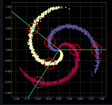
Spiral graph with Gaussian noise
The model image with Gaussian noise is closer to the real data
We can observe that the three samples in the graph are not linearly separable, and there are different samples for a certain region according to the linear division method
In order to solve this problem, we can use two ways, one is to transform the data into linearly separable through spatial transformation, and the other is to use neural network to obtain appropriate nonlinear data division
Construct spiral classification model
Each point in the two-dimensional coordinates is equivalent to a vector. There are three samples, and each sample has 1000 two-dimensional vectors
This is the input of the model. Construct a 3000 line 2-dimensional vector to construct the spiral space
And mark the corresponding category of each vector
X = torch.zeros(N * C, D).to(device)
Y = torch.zeros(N * C, dtype=torch.long).to(device)
for c in range(C):
    index = 0
    t = torch.linspace(0, 1, N) # Take 10000 numbers evenly between [0, 1] and assign them to t
    # The following code need not be understood too much. In short, three types of samples (which can form a spiral) are calculated according to the formula
    # torch.randn(N) is a group of random numbers with N mean values of 0 and variance of 1. Pay attention to distinguish it from rand
    inner_var = torch.linspace( (2*math.pi/C)*c, (2*math.pi/C)*(2+c), N) + torch.randn(N) * 0.2

    # The (x,y) coordinates of each sample are saved in X
    # The categories of samples stored in Y are [0, 1, 2]
    for ix in range(N * c, N * (c + 1)):
        X[ix] = t[index] * torch.FloatTensor((math.sin(inner_var[index]), math.cos(inner_var[index])))
        Y[ix] = c
        index += 1

print("Shapes:")
print("X:", X.size())
print("Y:", Y.size())
Construct linear model classification
Shape such as y = w x + b y=wx+b For the linear function of y=wx+b, if we use the linear function to train the data, we need a loss function calculation, and optimize our linear function through gradient back propagation
learning_rate = 1e-3
lambda_l2 = 1e-5

# The nn package is used to create a linear model
# Each linear model contains weight and bias
model = nn.Sequential(
    nn.Linear(D, H),
    nn.Linear(H, C)
)
model.to(device) # Put the model on the GPU

# nn contains many different loss functions. Here, the cross entropy loss function is used
criterion = torch.nn.CrossEntropyLoss()

# Here, optim package is used for stochastic gradient descent optimization
optimizer = torch.optim.SGD(model.parameters(), lr=learning_rate, weight_decay=lambda_l2)

# Start training
for t in range(1000):
    # Input the data into the model to get the prediction results
    y_pred = model(X)
    # Calculation loss and accuracy
    loss = criterion(y_pred, Y)
    score, predicted = torch.max(y_pred, 1)
    acc = (Y == predicted).sum().float() / len(Y)
    print('[EPOCH]: %i, [LOSS]: %.6f, [ACCURACY]: %.3f' % (t, loss.item(), acc))
    display.clear_output(wait=True)

    # Set the gradient to 0 before back propagation
    optimizer.zero_grad()
    # Back propagation optimization
    loss.backward()
    # Update all parameters
    optimizer.step()
We can see that in the code of the training part, we will calculate the loss and accuracy and output the corresponding parameters
In the process of back propagation, there is a gradient set to 0 operation, because PyTorch will accumulate the gradient by default (it is said that this is because it can reduce the requirements for GPU)
[EPOCH]: 999, [LOSS]: 0.864019, [ACCURACY]: 0.500
We can see that the accuracy is only 50%
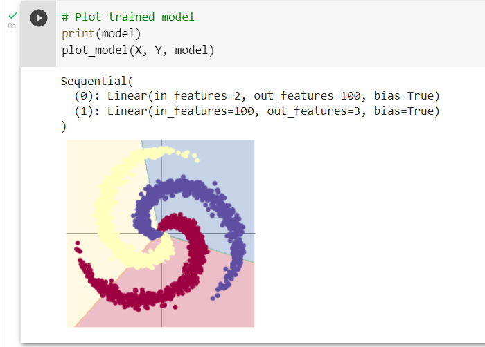
By observing the linear model, we can see that these two layers correspond to the two inputs of our model. The input of the first layer is the neural nodes of 100 samples, and the data used is the generated 3000 two-dimensional vectors. The second layer is our supervision data, that is, our corresponding manual division.
It can be seen that this is a simple linear model of supervised learning classification, and the division of this model can be seen from the figure that it is not very accurate
Adding activation function to construct two-layer neural network classification
learning_rate = 1e-3
lambda_l2 = 1e-5
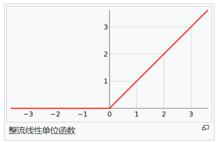
# It can be seen here that different from the above model, a ReLU activation function is added between the two layers
model = nn.Sequential(
nn.Linear(D, H),
nn.ReLU(),
nn.Linear(H, C)
)
model.to(device)
# The following code is exactly the same as before, but there is no more description here
criterion = torch.nn.CrossEntropyLoss()
optimizer = torch.optim.Adam(model.parameters(), lr=learning_rate, weight_decay=lambda_l2) # built-in L2
# The training model is exactly the same as the previous code
for t in range(1000):
y_pred = model(X)
loss = criterion(y_pred, Y)
score, predicted = torch.max(y_pred, 1)
acc = ((Y == predicted).sum().float() / len(Y))
print("[EPOCH]: %i, [LOSS]: %.6f, [ACCURACY]: %.3f" % (t, loss.item(), acc))
display.clear_output(wait=True)
# zero the gradients before running the backward pass.
optimizer.zero_grad()
# Backward pass to compute the gradient
loss.backward()
# Update params
optimizer.step()
It can be seen that we have added the ReLu() activation function to the two-tier model
Adding activation function means that the model has the ability to deal with nonlinear partition. We observe the results after training
It can be seen that the accuracy has been greatly improved
[EPOCH]: 999, [LOSS]: 0.178409, [ACCURACY]: 0.949
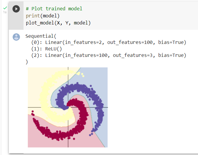
The number of layers of the model has also become an input layer and two processing neural networks. We can see that the division is at the local edge. Although there are still some inaccuracies, which may be caused by too little data, the overall accuracy has reached a very high level
reference material:
PyTorch study, frontier theory group, Vision Laboratory, Ocean University of China