Decision tree regression

Core idea: similar inputs will produce similar outputs. For example, predict someone's salary:

Age: 1-young, 2-middle-aged, 3-old Education: 1-bachelor, 2-master, 3-doctor Experience: 1-debut, 2-general, 3-veteran, 4-ashes Gender: 1-male, 2-female

The number of samples is very large 100 W Samples

Change a data structure to improve the retrieval efficiency

tree structure

Regression: mean
 Category: voting(probability)

In order to improve the search efficiency, the tree data structure is used to process the sample data:

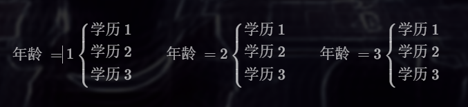
Firstly, select a feature from the training sample matrix to divide the sub table, so that the values of the feature in each sub table are all the same, then select the next feature in each sub table, continue to divide smaller sub tables according to the same rules, and repeat until all the features are used up. At this time, the leaf level sub table is obtained, in which the feature values of all samples are all the same. For the sample to be predicted, select the corresponding sub table according to the value of each feature and match it one by one until the leaf level sub table that exactly matches it is found. Use the output of the samples in the sub table to provide the output for the sample to be predicted through average (regression) or voting (classification).

Firstly, which feature is selected to partition the sub table determines the performance of the decision tree. With so many features, which feature is used to divide the row sub table first?

The bottom layer of the decision tree provided by sklearn is the cart tree (Classification and Regression Tree). The steps of cart regression tree in solving regression problems are as follows:

1. The original data set S, where the depth of the tree is depth=0;
2. For set S, traverse each value of each feature (traverse all discrete values in the data (12)) Use this value to split the original data set S into two sets: the left set (< = value samples) and the right set (> value samples), Calculate the MSE (mean square error) of the two sets respectively, find the value that minimizes (left_mse+right_mse), and record the feature name and value at this time. This is the best segmentation feature and the best segmentation value; ​ mse: mean square error ​ ((y1-y1')^2 + (y2-y2')^2 + (y3-y3')^2 + (y4-y4')^2 ) / 4 = mse

x1 y1 y1'

x2 y2 y2'

x3 y3 y3'

x4 y4 y4'

1. After finding the best segmentation feature and the best segmentation value, use the value to split the set S into two sets, depth+=1;
2. Repeat steps 2 and 3 respectively for the sets left and right until the termination conditions are met.

The underlying structure of decision tree is binary tree

The termination conditions are as follows:
1,Features have been used up: if there are no features available for use, the tree will stop splitting;
2,There are no samples in the child node: at this time, the node has no samples to divide, and the node stops splitting;
3,The tree has reached the preset maximum depth: depth >= max_depth，The tree stopped splitting.
4,The sample quantity of the node has reached the artificially set threshold: sample quantity < min_samples_split ，Then the node stops splitting;

API related to decision tree regressor model:

import sklearn.tree as st

# Create a decision tree regressor model. The maximum depth of the decision tree is 4
model = st.DecisionTreeRegressor(max_depth=4)
# Training model  
# train_x: Two dimensional array sample data
# train_y: Results corresponding to each row of samples in the training set
model.fit(train_x, train_y)
# test model 
pred_test_y = model.predict(test_x)

Case: predicting housing prices in the Boston area.

1. Read the data and interrupt the original data set. Divide training set and test set.

import sklearn.datasets as sd
import sklearn.utils as su
# Load Boston area house price dataset
boston = sd.load_boston()
print(boston.feature_names)
# |CRIM|ZN|INDUS|CHAS|NOX|RM|AGE|DIS|RAD|TAX|PTRATIO|B|LSTAT|
# Crime rate | proportion of residential land | proportion of commercial land | whether it depends on the river | air quality | number of rooms | service life | distance from the central area | road network density | real estate tax | teacher-student ratio | proportion of blacks | proportion of low status population|
# Disrupt the input and output of the original data set
x, y = su.shuffle(boston.data, boston.target, random_state=7)
# Divide training set and test set
train_size = int(len(x) * 0.8)
train_x, test_x, train_y, test_y = \
    x[:train_size], x[train_size:], \
    y[:train_size], y[train_size:]

1. Create a decision tree regressor model and use the training set to train the model. Test the model using a test set.

import sklearn.tree as st
import sklearn.metrics as sm

# Create decision tree regression model
model = st.DecisionTreeRegressor(max_depth=4)
# Training model
model.fit(train_x, train_y)
# test model 
pred_test_y = model.predict(test_x)
print(sm.r2_score(test_y, pred_test_y))

Integration algorithm

Three cobblers make Zhuge Liang

The prediction results obtained by a single model are always one-sided. According to the prediction results given by multiple different models, the final prediction results are obtained by means of average (regression) or voting (classification).

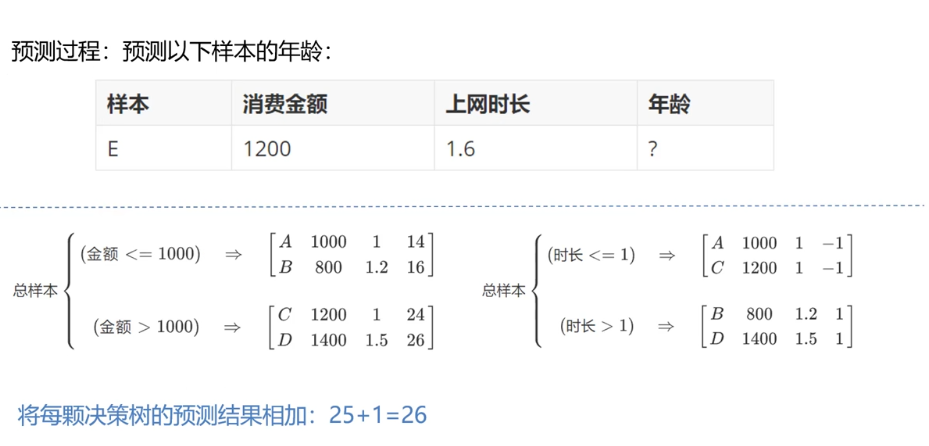
The integration algorithm based on decision tree is to build multiple different decision tree models according to certain rules, give the prediction results for unknown samples respectively, and finally get a relatively comprehensive conclusion through average or voting. Common integration models include Boosting class models (AdaBoost, GBDT XGBoost )And Bagging (self-help aggregation, random forest) model.

AdaBoost model (positive excitation)

Firstly, the samples in the sample matrix are randomly assigned initial weights, so as to build a decision tree with weights. When the decision tree provides prediction output, the prediction value is generated by weighted average or weighted voting.

A decision tree has been built and all female doctors have been found through 1322. One of them is 6000, 8000, 9000 and 10000
 Due to the positive excitation, each sample is assigned an initial weight of:1 1 1 3  Forecast: weighted average

The training samples are substituted into the model to predict its output. For those samples whose predicted value is different from the actual value, the weight is improved and targeted training is carried out, so as to form the second decision tree. Repeat the above process to build several decision trees with different weights.

Actual value: 10000, but you predicted to build a second decision tree for 6000 and increase the weight of 10000 samples

API related to positive excitation:

import sklearn.tree as st
import sklearn.ensemble as se
# Model: decision tree model (one)
model = st.DecisionTreeRegressor(max_depth=4)
# Adaptive enhanced decision tree regression model	
# 
model = se.AdaBoostRegressor(model, n_estimators=400, random_state=7)

Basic model of positive incentive: Decision Tree
n_estimators: Build 400 decision trees with different weights and train the model

# Training model
model.fit(train_x, train_y)
# test model 
pred_test_y = model.predict(test_x)

Case: a model for predicting housing prices in Boston based on positive incentive training.

# Create a positive incentive regressor model based on decision tree
model = se.AdaBoostRegressor(
	st.DecisionTreeRegressor(max_depth=4), n_estimators=400, random_state=7)
# Training model
model.fit(train_x, train_y)
# test model 
pred_test_y = model.predict(test_x)
print(sm.r2_score(test_y, pred_test_y))

Characteristic importance

As a by-product of the training process of decision tree model, the importance of the feature is marked according to the order of selecting the feature when dividing the sub table, which is the importance index of the feature. The trained model object provides the attribute: feature_importances_ To store the importance of each feature.

Obtain the characteristic importance attribute of the sample matrix:

model.fit(train_x, train_y)
fi = model.feature_importances_

Case: obtain the eigenvalues of the two models trained by ordinary decision tree and positive incentive decision tree, and output the drawing in the order from large to small.

import matplotlib.pyplot as mp

model = st.DecisionTreeRegressor(max_depth=4)
model.fit(train_x, train_y)
# The feature importance given by the decision tree regressor
fi_dt = model.feature_importances_
model = se.AdaBoostRegressor(
    st.DecisionTreeRegressor(max_depth=4), n_estimators=400, random_state=7)
model.fit(train_x, train_y)
# The characteristic importance given by the forward incentive regressor based on decision tree
fi_ab = model.feature_importances_

mp.figure('Feature Importance', facecolor='lightgray')
mp.subplot(211)
mp.title('Decision Tree', fontsize=16)
mp.ylabel('Importance', fontsize=12)
mp.tick_params(labelsize=10)
mp.grid(axis='y', linestyle=':')
sorted_indices = fi_dt.argsort()[::-1]
pos = np.arange(sorted_indices.size)
mp.bar(pos, fi_dt[sorted_indices], facecolor='deepskyblue', edgecolor='steelblue')
mp.xticks(pos, feature_names[sorted_indices], rotation=30)
mp.subplot(212)
mp.title('AdaBoost Decision Tree', fontsize=16)
mp.ylabel('Importance', fontsize=12)
mp.tick_params(labelsize=10)
mp.grid(axis='y', linestyle=':')
sorted_indices = fi_ab.argsort()[::-1]
pos = np.arange(sorted_indices.size)
mp.bar(pos, fi_ab[sorted_indices], facecolor='lightcoral', edgecolor='indianred')
mp.xticks(pos, feature_names[sorted_indices], rotation=30)
mp.tight_layout()
mp.show()

GBDT

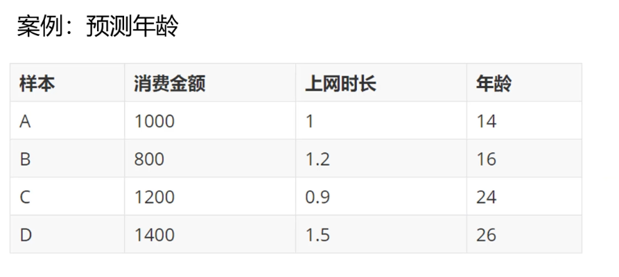
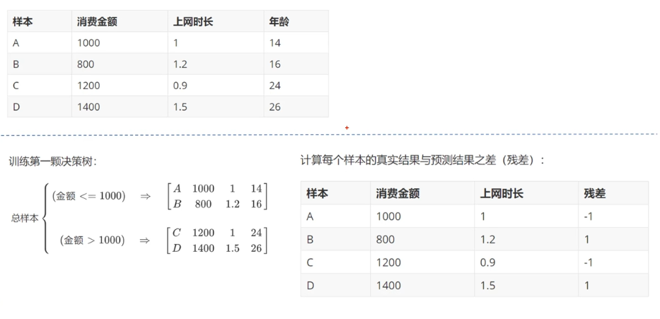
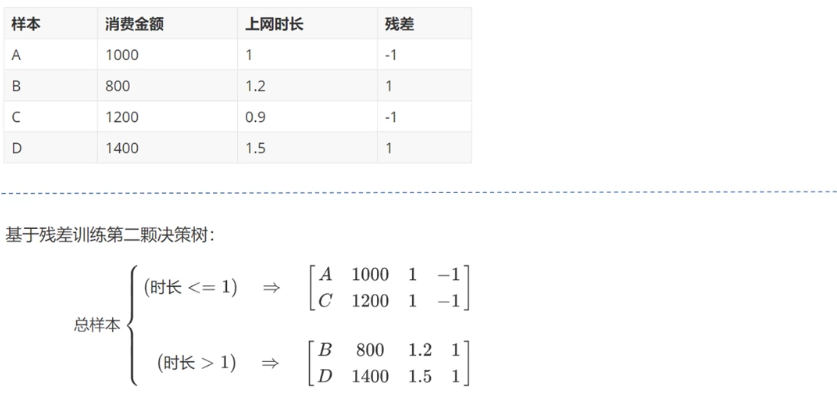
GBDT (Gradient Boosting Decision Tree) generates a weak classifier through multiple rounds of iterations. Each classifier is trained based on the residual * * (residual refers to the difference between the actual observed value and the estimated value (fitting value) in Mathematical Statistics) * * of the previous round of classifier. Design the loss function based on the residual of the prediction results. The process of GBDT training is the process of finding the minimum value of the loss function.

case

Principle 1:

Principle 2:

Principle 3:

import sklearn.tree as st
import sklearn.ensemble as se
# Adaptive enhanced decision tree regression model	
# n_estimators: build 400 decision trees with different weights and train the model
model = se.GridientBoostingRegressor(
    	max_depth=10, n_estimators=1000, min_samples_split=2)
# Training model
model.fit(train_x, train_y)
# test model 
pred_test_y = model.predict(test_x)

Self service aggregation (BootStrap)

Each time, some samples are randomly selected from the total sample matrix in the way of put back sampling to build a decision tree, so as to form multiple decision trees containing different training samples, so as to weaken the impact of some strong samples on the prediction results of the model and improve the generalization characteristics of the model.

Because most of the training of sklean has been packaged into interfaces, it is difficult to adjust the samples of each training, so self-service aggregation is not easy to use without sklean interface.

Random forest

On the basis of self-help aggregation, each time the decision tree model is constructed, not only some samples but also some features are randomly selected. This set algorithm not only avoids the influence of strong samples on the prediction results, but also weakens the influence of strong features, making the prediction ability of the model more generalized.

Random forest related API:

import sklearn.ensemble as se
# Stochastic Forest regression model 	 (belonging to a set algorithm)
# max_depth: maximum depth of decision tree 10
# n_estimators: build 1000 decision trees and train models
# min_samples_split: if the minimum number of samples in the sub table is less than this number, it will not continue to split down
model = se.RandomForestRegressor(
    max_depth=10, n_estimators=1000, min_samples_split=2)

Case: analyze the demand for shared bicycles, so as to judge how to launch shared bicycles.

1. Load and organize datasets
2.feature analysis 
3.Disrupt data set, divide training set and test set

import numpy as np
import sklearn.utils as su
import sklearn.ensemble as se
import sklearn.metrics as sm
import matplotlib.pyplot as mp

data = np.loadtxt('../data/bike_day.csv', unpack=False, dtype='U20', delimiter=',')
day_headers = data[0, 2:13]
x = np.array(data[1:, 2:13], dtype=float)
y = np.array(data[1:, -1], dtype=float)

x, y = su.shuffle(x, y, random_state=7)
print(x.shape, y.shape)
train_size = int(len(x) * 0.9)
train_x, test_x, train_y, test_y = \
    x[:train_size], x[train_size:], y[:train_size], y[train_size:]
# Random forest regressor
model = se.RandomForestRegressor( max_depth=10, n_estimators=1000, min_samples_split=2)
model.fit(train_x, train_y)
# Feature importance based on "day" dataset
fi_dy = model.feature_importances_
pred_test_y = model.predict(test_x)
print(sm.r2_score(test_y, pred_test_y))

data = np.loadtxt('../data/bike_hour.csv', unpack=False, dtype='U20', delimiter=',')
hour_headers = data[0, 2:13]
x = np.array(data[1:, 2:13], dtype=float)
y = np.array(data[1:, -1], dtype=float)
x, y = su.shuffle(x, y, random_state=7)
train_size = int(len(x) * 0.9)
train_x, test_x, train_y, test_y = \
    x[:train_size], x[train_size:], \
    y[:train_size], y[train_size:]
# Random forest regressor
model = se.RandomForestRegressor(
    max_depth=10, n_estimators=1000,
    min_samples_split=2)
model.fit(train_x, train_y)
# Feature importance based on "hour" dataset
fi_hr = model.feature_importances_
pred_test_y = model.predict(test_x)
print(sm.r2_score(test_y, pred_test_y))

The drawing shows the characteristic importance of two sets of sample data:

mp.figure('Bike', facecolor='lightgray')
mp.subplot(211)
mp.title('Day', fontsize=16)
mp.ylabel('Importance', fontsize=12)
mp.tick_params(labelsize=10)
mp.grid(axis='y', linestyle=':')
sorted_indices = fi_dy.argsort()[::-1]
pos = np.arange(sorted_indices.size)
mp.bar(pos, fi_dy[sorted_indices], facecolor='deepskyblue', edgecolor='steelblue')
mp.xticks(pos, day_headers[sorted_indices], rotation=30)

mp.subplot(212)
mp.title('Hour', fontsize=16)
mp.ylabel('Importance', fontsize=12)
mp.tick_params(labelsize=10)
mp.grid(axis='y', linestyle=':')
sorted_indices = fi_hr.argsort()[::-1]
pos = np.arange(sorted_indices.size)
mp.bar(pos, fi_hr[sorted_indices], facecolor='lightcoral', edgecolor='indianred')
mp.xticks(pos, hour_headers[sorted_indices], rotation=30)
mp.tight_layout()
mp.show()

Supplementary knowledge

Detailed calculation of R2 coefficient

The detailed calculation process of R2 coefficient is as follows:

If y is used_ I represents the real observed value, with \ bar{y} representing the average value of the real observed value and \ hat{y_i} representing the predicted value, then there are the following evaluation indicators:

• Regression sum of squares (SSR)

SSR = \sum_{i=1}^{n}(\hat{y_i} - \bar{y})^2

The error between the estimated value and the average value reflects the sum of squares of the deviation of the correlation degree between the independent variable and the dependent variable

• Sum of squares of residuals (SSE)

SSE = \sum_{i=1}^{n}(y_i-\hat{y_i} )^2

That is, the error between the estimated value and the real value reflects the fitting degree of the model

• Sum of squares of total deviations (SST)

SST =SSR + SSE= \sum_{i=1}^{n}(y_i - \bar{y})^2

That is, the error between the average value and the real value reflects the deviation from the mathematical expectation

• R2_score calculation formula

R2_score, that is, the coefficient of determination, reflects the proportion that all variations of dependent variables can be explained by independent variables through regression relationship Calculation formula:

R^2=1-\frac{SSE}{SST}

Namely:

R^2 = 1 - \frac{\sum_{i=1}^{n} (y_i - \hat{y}_i)2}{\sum_{i=1}{n} (y_i - \bar{y})^2}

Further simplified as:

R^2 = 1 - \frac{\sum\limits_i(y_i - y_i)^2 / n}{\sum\limits_i(y_i - \hat{y})^2 / n} = 1 - \frac{RMSE}{Var}

If the error is larger than the mean value or the numerator of the error is smaller than the numerator ^ 2, it can be understood that if the error is smaller than the numerator ^ 2, it can be used as the evaluation index

R2_score = 1, the predicted value and the real value in the sample are completely equal without any error, which means that the better the interpretation of the independent variable to the dependent variable in the regression analysis

R2_score = 0, the numerator is equal to the denominator, and each predicted value of the sample is equal to the mean

Derivation process of linear regression loss function

The linear function is defined as:

y = w_0 + w_0 x_1

Adopt the mean square loss function:

loss = \frac{1}{2} (y - y')^2

Where y is the true value from the sample; Y 'is the predicted value, that is, the expression of linear equation, which is brought into the loss function to obtain:

loss = \frac{1}{2} (y - (w_0 + w_1 x_1))^2

Expand the formula:

loss = \frac{1}{2} (y^2 - 2y(w_0 + w_1 x_1) + (w_0 + w_1 x_1)^2) \\ \frac{1}{2} (y^2 - 2y*w_0 - 2y*w_1x_1 + w_0^2 + 2w_0*w_1 x_1 + w_1^2x_1^2) \\

Right w_0 # derivation:

\frac{\partial loss}{\partial w_0} = \frac{1}{2}(0-2y-0+2w_0 + 2w_1 x_1 +0) \\ =\frac{1}{2}(-2y + 2 w_0 + 2w_1 x_1) \\ = \frac{1}{2} * 2(-y + (w_0 + w_1 x_1)) \\ =(-y + y') = -(y - y')

Right w_1. Derivation:

\frac{\partial loss}{\partial w_1} = \frac{1}{2}(0-0-2y*x_1+0+2 w_0 x_1 + 2 w_1 x_1^2) \\ = \frac{1}{2} (-2y x_1 + 2 w_0 x_1 + 2w_1 x_1^2) \\ = \frac{1}{2} * 2 x_1(-y + w_0 + w_1 x_1) \\ = x_1(-y + y') = - x_1(y - y')

The derivation is complete