linear model

Linear model is one of the simplest models in nature. It describes that the influence of one (or more) independent variable on another dependent variable is in a simple proportional and linear relationship For example:

• The unit price of housing is 10000 yuan per square meter, 1 million yuan for 100 square meters and 1.2 million yuan for 120 square meters;
• An excavator can dig 100m^3 sand every hour, and it can dig 400m^3 sand in 4 hours

The linear model is represented as a straight line in two-dimensional space and a plane in three-dimensional space. The linear model in higher dimensions is difficult to be represented by geometry (called hyperplane) As shown in the figure below:

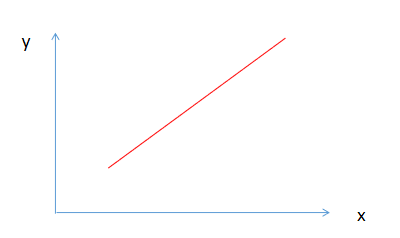
The linear model is represented as a straight line in two-dimensional space

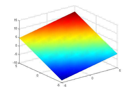
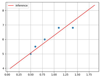
The linear model in three-dimensional space is expressed as a plane linear regression, which is to find a linear model according to a set of input and output values (called samples), which can best fit the given numerical distribution, so as to predict the output when a new input is given The sample is shown in the following table:

The linear model fitted according to the sample is shown in the figure below:

Linear model definition

Given a set of attributes x, x=(x_1;x_2;...;x_n), the general expression of linear equation is:

y = w_1x_1 + w_2x_2 + w_3x_3 + ... + w_nx_n + b

Written in vector form:

y=wTx+by = w^Tx + b y=wTx+b

Where, w=(w_1;w_2;...;w_n), x=(x_1;x_2;...;x_n), W and b can be determined after learning When the number of independent variables is 1, the above linear model is the linear equation under the plane:

y=wx+b

Linear model is simple and easy to model, but it contains some important basic ideas in machine learning Many powerful nonlinear models can be derived by introducing hierarchy or high-dimensional mapping based on linear models In addition, because www intuitively expresses the importance of each attribute in prediction, the linear model has good interpretability For example, to judge whether a watermelon is a good one, you can use the following expression:

f_{\text {good melon}} (x) = 0.2x_{\text {color}} + 0.5x_{\text {root}} + 0.3x_{\text {knock}} + 1

The above formula can be explained that whether a watermelon is a good melon can be judged by color, root, knocking sound and other factors, among which the root is the most important (with the highest weight), followed by knocking sound and color

model training

In a two - dimensional plane, given two points, a straight line can be determined However, in practical engineering, there may be many sample points, and a straight line cannot be found to accurately pass through all sample points. Only a straight line "close enough" or "small enough" to the sample can be found to approximate the given sample. As shown in the figure below:

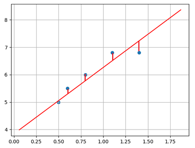
How do you determine that the straight line is close enough to all samples? The loss function can be used for measurement

loss function

The loss function is used to measure the difference between the real value (given in the sample) and the predicted value (calculated by the model) The smaller the value of the loss function, the smaller the difference between the predicted value and the real value of the model, and the better the performance of the model; The larger the loss function, the greater the difference between the predicted value and the real value of the model, and the worse the performance of the model In regression problems, mean square deviation is a commonly used loss function, and its expression is as follows:

E = \frac{1}{2}\sum_{i=1}^{n}{(y - y')^2}

Where, y is the predicted value of the model and y 'is the real value Euclidean distance has a very good geometric meaning The task of linear regression is to find the optimal linear model, which is to minimize the value of loss function, that is:

(w^*, b^*) = arg min \frac{1}{2}\sum_{i=1}^{n}{(y - y')^2} \\ = arg min \frac{1}{2}\sum_{i=1}^{n}{(y' - wx_i - b)^2}

The method of solving the model based on the minimization of mean square error is called "least square method" In linear regression, the least square method is trying to find a straight line, which is the minimum sum of the Euclidean distances from all samples to the straight line The loss function can be derived from w and b respectively to obtain the derivative of the loss function, and the optimal solution of w and b can be obtained by making the derivative 0

Gradient descent method

Why use gradient descent

In practical calculation, there are some problems in solving the optimal parameters by the least square method:

(1) The least square method needs to calculate the inverse matrix, which may not exist;

(2) When the number of sample features is large, the calculation of inverse matrix is very time-consuming or even infeasible

Therefore, in practical calculation, the gradient descent method is usually used to solve the minimum value of the loss function, so as to find the optimal parameters of the model

What is gradient descent

Gradient is a vector (vector with direction), which indicates that the directional derivative of a function at the point gets the maximum value along the direction, that is, the function changes the fastest and the change rate is the largest along the direction (the direction of the gradient) at the point The loss function converges fastest in the opposite direction of the gradient (i.e. the extreme point can be found fastest) When the gradient vector is zero (or close to zero), it indicates that it reaches an extreme point, which is also the termination condition of iterative calculation of gradient descent algorithm

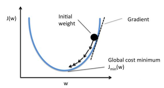
This process of constantly adjusting the weight of the function according to the negative gradient is called "gradient descent method" In this way, changing the weight makes the value of the loss function drop faster, and then the value converges to a minimum of the loss function

Through the loss function, we transform the problem of "finding the optimal parameter" into the problem of "finding the minimum value of the loss function" The gradient descent algorithm is described as follows:

(1) Is the loss small enough? If not, calculate the gradient of the loss function (2) Take a small step in the opposite direction of the gradient to reduce the loss (3) Cycle to (1)

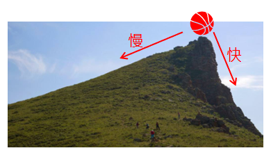
In the gradient descent method, the parameters are continuously adjusted along the negative direction of the gradient, so as to gradually approach the minimum point of the loss function As shown in the figure below:

Parameter update rule

In the linear equation, there are two parameters to learn, w_0 and w_1. In the process of gradient descent, these two parameters are adjusted separately. The adjustment rule is as follows: w_0 = w_0 + \Delta w_0\ w_1 = w_1 + \Delta w_ one

\Delta w_0 and \ Delta w_1 can be expressed as:

\Delta w_0 = -\eta \frac{\Delta loss}{\Delta w_0}\\ \Delta w_1 = -\eta \frac{\Delta loss}{\Delta w_1}\\

Among them, η It is called the learning rate, and \ frac{\Delta loss}{\Delta w_i} is the gradient (i.e. the partial derivative of the loss function with respect to the parameter w_i) The expression of loss function is:

loss =\frac{1}{2}\sum(y - y')^2 = \frac{1}{2}\sum((y-(w_0+w_1x))^2)

By deriving the loss function (see Supplementary knowledge for the derivation process), we can get W_ 0, w_ The partial derivative of 1 is:

\frac{\Delta loss}{\Delta w_0} = \sum((y - y')(-1)) = -\sum(y - y')\\ \frac{\Delta loss}{\Delta w_1} = \sum((y - y')(-x)) = -\sum(x(y - y'))

Realize linear regression

Self coding implementation

The following is the code to realize linear regression:

# Linear regression example
import numpy as np
import matplotlib.pyplot as mp
from mpl_toolkits.mplot3d import axes3d
import sklearn.preprocessing as sp

# Training data set
train_x = np.array([0.5, 0.6, 0.8, 1.1, 1.4])  # Input set
train_y = np.array([5.0, 5.5, 6.0, 6.8, 7.0])  # Output set

n_epochs = 1000  # Number of iterations
lrate = 0.01  # Learning rate
epochs = []  # Record the number of iterations
losses = []  # Record loss value

w0, w1 = [1], [1]  # Model initial value

for i in range(1, n_epochs + 1):
    epochs.append(i)  # Record the number of iterations

    y = w0[-1] + w1[-1] * train_x  # Take out the latest W0 and W1 and calculate the linear equation output
    # Mean loss function
    loss = (((train_y - y) ** 2).sum()) / 2
    losses.append(loss)  # Record the loss value of each iteration

    print("%d: w0=%f, w1=%f, loss=%f" % (i, w0[-1], w1[-1], loss))

    # Calculate the partial derivatives of W0 and W1
    d0 = -(train_y - y).sum()
    d1 = -(train_x * (train_y - y)).sum()

    # Update w0,w1
    w0.append(w0[-1] - (d0 * lrate))
    w1.append(w1[-1] - (d1 * lrate))

Program execution results:

1 w0=1.00000000 w1=1.00000000 loss=44.17500000
2 w0=1.20900000 w1=1.19060000 loss=36.53882794
3 w0=1.39916360 w1=1.36357948 loss=30.23168666
4 w0=1.57220792 w1=1.52054607 loss=25.02222743
5 w0=1.72969350 w1=1.66296078 loss=20.71937337
......
996 w0=4.06506160 w1=2.26409126 loss=0.08743506
997 w0=4.06518850 w1=2.26395572 loss=0.08743162
998 w0=4.06531502 w1=2.26382058 loss=0.08742820
999 w0=4.06544117 w1=2.26368585 loss=0.08742480
1000 w0=4.06556693 w1=2.26355153 loss=0.08742142

You can add visualization to the data to make the results more intuitive Add the following code:

###################### Visualization of training process ######################
# Visualization of training process
## Convergence process of loss function
w0 = np.array(w0[:-1])
w1 = np.array(w1[:-1])

mp.figure("Losses", facecolor="lightgray")  # Create a form
mp.title("epoch", fontsize=20)
mp.ylabel("loss", fontsize=14)
mp.grid(linestyle=":")  # Gridlines: dashed lines
mp.plot(epochs, losses, c="blue", label="loss")
mp.legend()  # legend
mp.tight_layout()  # Compact format

## Display model lines
pred_y = w0[-1] + w1[-1] * train_x  # Predict y based on x
mp.figure("Linear Regression", facecolor="lightgray")
mp.title("Linear Regression", fontsize=20)
mp.xlabel("x", fontsize=14)
mp.ylabel("y", fontsize=14)
mp.grid(linestyle=":")
mp.scatter(train_x, train_y, c="blue", label="Traing")  # Draw sample scatter diagram
mp.plot(train_x, pred_y, c="red", label="Regression")
mp.legend()

# Display gradient descent process (copy and paste, no need to write)
# Loss function on the surface (WF = loss function 1)
arr1 = np.linspace(0, 10, 500)  # A uniform list of 500 elements is generated between 0 and 9
arr2 = np.linspace(0, 3.5, 500)  # A uniform list of 500 elements is generated between 0 and 3.5

grid_w0, grid_w1 = np.meshgrid(arr1, arr2)  # Generate two-dimensional matrix

flat_w0, flat_w1 = grid_w0.ravel(), grid_w1.ravel()  # Flattening of two-dimensional matrix
loss_metrix = train_y.reshape(-1, 1)  # The generated error matrix (- 1,1) represents the dimension calculated automatically
outer = np.outer(train_x, flat_w1)  # Find the outer product (a new matrix in which the elements of train_x and flat_w1 are multiplied by each other)
# Calculated loss: ((w0 + w1*x - y)**2)/2
flat_loss = (((flat_w0 + outer - loss_metrix) ** 2).sum(axis=0)) / 2
grid_loss = flat_loss.reshape(grid_w0.shape)

mp.figure('Loss Function')
ax = mp.gca(projection='3d')
mp.title('Loss Function', fontsize=14)
ax.set_xlabel('w0', fontsize=14)
ax.set_ylabel('w1', fontsize=14)
ax.set_zlabel('loss', fontsize=14)
ax.plot_surface(grid_w0, grid_w1, grid_loss, rstride=10, cstride=10, cmap='jet')
ax.plot(w0, w1, losses, 'o-', c='orangered', label='BGD', zorder=5)
mp.legend(loc='lower left')

mp.show()

The data visualization results are shown in the figure below:

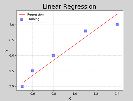
Linear model obtained by regression

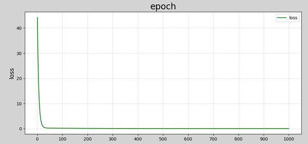
Convergence process of loss function

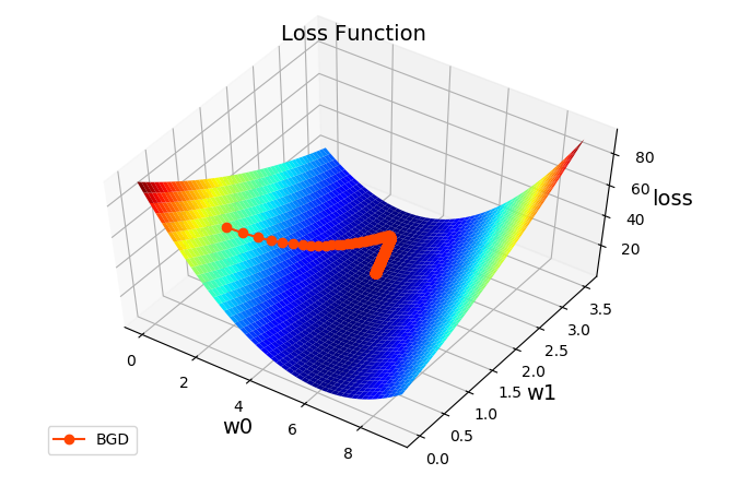
Gradient descent process

Implemented through sklearn API

Similarly, linear regression can be implemented using the API provided by sklearn library The code is as follows:

# Linear regression using linear regression
import numpy as np
import sklearn.linear_model as lm  # linear model# linear model
import sklearn.metrics as sm  # Model performance evaluation module
import matplotlib.pyplot as mp

train_x = np.array([[0.5], [0.6], [0.8], [1.1], [1.4]])  # Input set
train_y = np.array([5.0, 5.5, 6.0, 6.8, 7.0])  # Output set

# Create linear regressor
model = lm.LinearRegression()
# Training regressors with known input and output data sets
model.fit(train_x, train_y)
# Predict the output according to the training model
pred_y = model.predict(train_x)

print("coef_:", model.coef_)  # coefficient
print("intercept_:", model.intercept_)  # intercept

# Visual regression curve
mp.figure('Linear Regression', facecolor='lightgray')
mp.title('Linear Regression', fontsize=20)
mp.xlabel('x', fontsize=14)
mp.ylabel('y', fontsize=14)
mp.tick_params(labelsize=10)
mp.grid(linestyle=':')

# Draw sample points
mp.scatter(train_x, train_y, c='blue', alpha=0.8, s=60, label='Sample')

# Draw a fitting line
mp.plot(train_x,  # x coordinate data
        pred_y,  # y coordinate data
        c='orangered', label='Regression')

mp.legend()
mp.show()

Execution result:

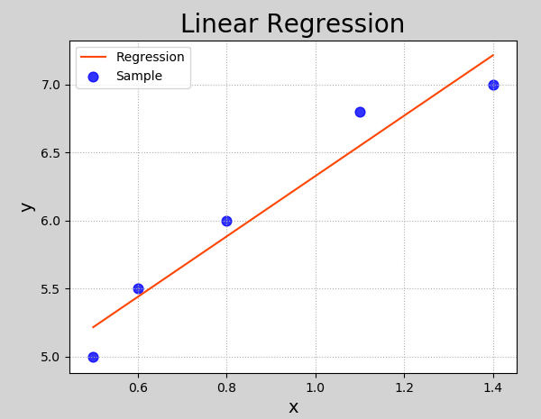
Model evaluation index

(1) Mean Absolute Deviation: the average of the absolute value of the deviation between a single observation value and the arithmetic mean;

(2) Mean square error: the square average of the difference between a single sample and the average value;

(3) Mad (median absolute deviation): the median value of the absolute deviation from the median value of the data;

(4) R2 determination coefficient: tends to 1, the better the model; If it tends to 0, the worse the model is

polynomial regression

What is polynomial regression

Linear regression is applicable to the regression problem in which the data are linearly distributed If the data samples show obvious nonlinear distribution, the linear regression model is no longer applicable (left in the figure below), but polynomial regression may be better (right in the figure below) For example:

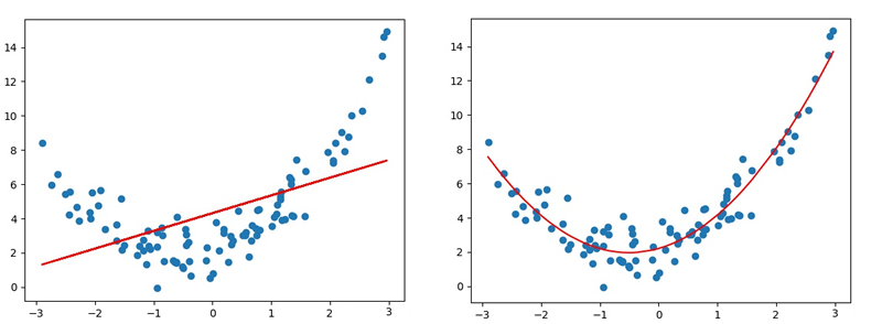
Polynomial model definition

Compared with the linear model, the polynomial model introduces a higher-order term, and the exponent of the independent variable is greater than 1, such as the univariate quadratic equation:

y = w_0 + w_1x + w_2x^2

Univariate cubic equation:

y = w_0 + w_1x + w_2x^2 + w_3x ^ 3

Extended to univariate nth order equation:

y = w_0 + w_1x + w_2x^2 + w_3x ^ 3 + ... + w_nx^n

The above expression can be simplified to:

y = \sum_{i=1}^N w_ix^i

Relationship with linear regression

Polynomial regression can be understood as an extension of linear regression, adding new eigenvalues to the linear regression model For example, to predict the price of a house, there is x_1, x_2, x_3. Three eigenvalues, which respectively represent the length, width and height of the house, can be expressed as the following linear model:

y = w_1 x_1 + w_2 x_2 + w_3 x_3 + b

For the house price, you can also use the volume of the house instead of using X directly_ 1, x_ 2, x_ 3. Three features:

y = w_0 + w_1x + w_2x^2 + w_3x ^ 3

Equivalent to creating a new feature x,x = length * width * height The above two models can be explained as follows:

• House price is a linear model of three characteristics: length, width and height
• House price is a polynomial model of volume

Therefore, the univariate polynomial of degree n can be transformed into a linear model of degree n

Polynomial regression implementation

For univariate n-degree polynomials, the method of minimizing the loss value by gradient descent can also be used to find the optimal model parameter w_0, w_1, w_2, ..., w_n​. The univariate polynomial of degree n can be transformed into a polynomial of degree n to obtain linear regression The following is an implementation of polynomial regression

# Polynomial regression example
import numpy as np
# linear model
import sklearn.linear_model as lm
# Model performance evaluation module
import sklearn.metrics as sm
import matplotlib.pyplot as mp
# Pipeline module
import sklearn.pipeline as pl
import sklearn.preprocessing as sp

train_x, train_y = [], []   # Input and output samples
with open("poly_sample.txt", "rt") as f:
    for line in f.readlines():
        data = [float(substr) for substr in line.split(",")]
        train_x.append(data[:-1])
        train_y.append(data[-1])

train_x = np.array(train_x)  # Input matrix in the form of two-dimensional data, with one sample per row and one feature per column
train_y = np.array(train_y)  # An output sequence in the form of a one-dimensional array. Each element corresponds to an input sample
# print(train_x)
# print(train_y)

# The polynomial feature is extended to preprocess and connected in series with a linear regressor to form a pipeline
# Polynomial feature extension: a transformation of existing data by mapping the data to a higher dimensional space
# After polynomial expansion, we can think that the model has changed from a straight line to a curve
# So we can fit the data more flexibly
# pipeline connects two models
model = pl.make_pipeline(sp.PolynomialFeatures(3), # Polynomial feature extension, the highest degree of extension is 3
                         lm.LinearRegression())

# Training regressors with known input and output data sets
model.fit(train_x, train_y)
# print(model[1].coef_)
# print(model[1].intercept_)

# Predict the output according to the training model
pred_train_y = model.predict(train_x)

# Evaluation index
err4 = sm.r2_score(train_y, pred_train_y)  # R2 score, range [0, 1], the greater the score, the better
print(err4)

# Build test sets outside the training set
test_x = np.linspace(train_x.min(), train_x.max(), 1000)
pre_test_y = model.predict(test_x.reshape(-1, 1)) # Predict new samples

# Visual regression curve
mp.figure('Polynomial Regression', facecolor='lightgray')
mp.title('Polynomial Regression', fontsize=20)
mp.xlabel('x', fontsize=14)
mp.ylabel('y', fontsize=14)
mp.tick_params(labelsize=10)
mp.grid(linestyle=':')
mp.scatter(train_x, train_y, c='dodgerblue', alpha=0.8, s=60, label='Sample')

mp.plot(test_x, pre_test_y, c='orangered', label='Regression')

mp.legend()
mp.show()

Printout:

0.9224401504764776

Execution result:

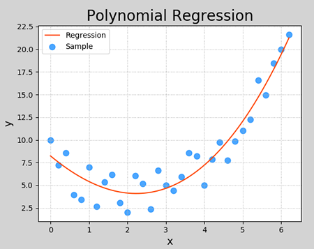
Over fitting and under fitting

What are under fitting and over fitting

In the example of polynomial regression in the previous section, the multinomial feature expander PolynomialFeatures() specifies a maximum degree of 3 when performing polynomial expansion. This parameter is an important parameter of polynomial expansion. If it is not selected properly, it may lead to different fitting effects The following figure shows the fitted image of the model when the parameter is set to 1 and 20 respectively:

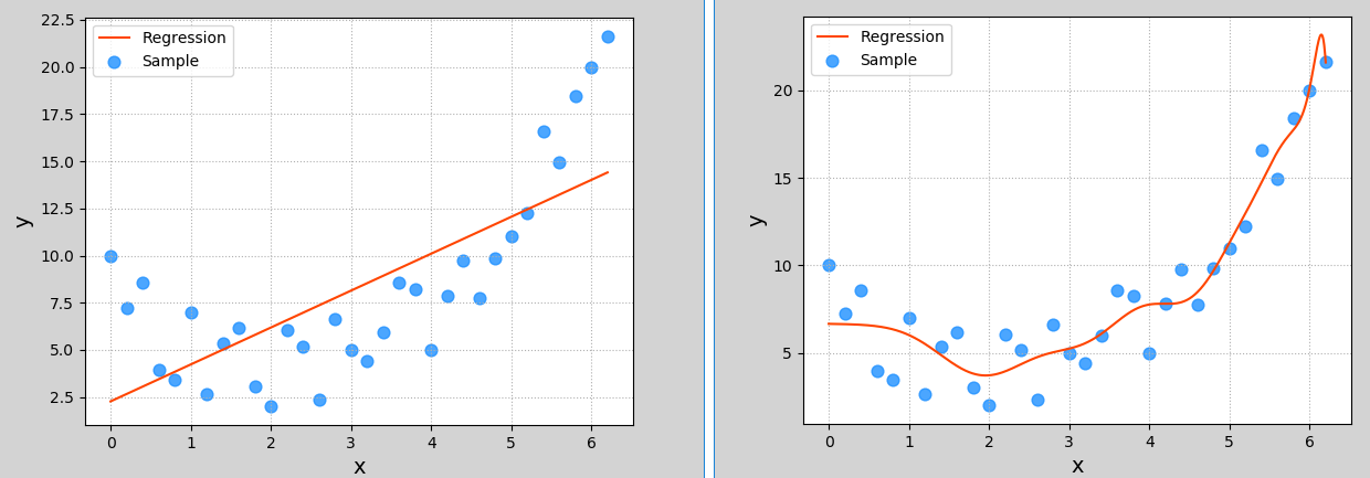
Neither of these is a good model The former does not learn the data distribution law, the degree of model fitting is not enough, and the prediction accuracy is too low. This phenomenon is called "under fitting"; The latter fits more samples too much, so that the generalization ability of the model (the adaptability of new samples) becomes worse. This phenomenon is called "over fitting"** Under fitting model generally shows that the accuracy of training set and test set is relatively low; The over fitting model generally has higher accuracy in the training set and lower accuracy in the test set** A good model, whether for training data or test data, has close prediction accuracy, and the accuracy should not be too low

[thinking 1] which of the following models is better, which is worse, and why?

[answer] the first model is not fitted; The second model is over fitted; The third model is moderate and acceptable

[thinking 2] which of the following curves is under fitting or over fitting, and which model fits best?

[answer] the first model is not fitted; The third model is over fitted; The second model fits well

How to deal with under fitting and over fitting

• Under fitting: improve the complexity of the model, such as adding features, increasing the highest power of the model, etc;
• Over fitting: reduce the complexity of the model, such as reducing features, reducing the highest power of the model, and so on

Variants of linear regression model

Another common reason for over fitting is that the model parameter value is too large, so the over fitting problem can be solved by inhibiting the parameters As shown in the following figure, the right figure produces a certain degree of over fitting, which can be reduced by weakening the coefficient of the higher-order term (but not deleting it)

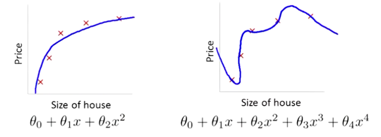
For example, in \ theta_3, \theta_4. Add certain coefficients to suppress the coefficients of these two higher-order terms. This method is called regularization. However, in practical problems, there may be more coefficients, and we don't know which coefficients should be suppressed. Therefore, we can avoid over fitting by shrinking all coefficients

Regularization definition

Regularization refers to the means of adding a norm after the objective function (such as loss function) to prevent over fitting. This norm is defined as:

||x||_p = (\sum_{i=1}^N |x|^p)^{\frac{1}{p}}

When p=1, it is called L1 norm (i.e. the sum of absolute values of all coefficients):

||x||_1 = (\sum_{i=1}^N |x|)

When p=2 is, it is called L2 norm (i.e. the square of the sum of all coefficients):

||x||_2 = (\sum_{i=1}^N |x|^2)^{\frac{1}{2}}

By adding regular terms to the objective function, the size of the parameters is compressed as a whole, so as to prevent over fitting

Lasso regression and ridge regression

Lasso regression and Ridge Regression modify the regression algorithm of loss function on the basis of standard linear regression Lasso regression is fully called Least absolute shrinkage and selection operator, which also translates into "minimum absolute value convergence and selection operator" and "lasso algorithm". Its loss function is as follows:

E = \frac{1}{n}(\sum_{i=1}^N y_i - y_i')^2 + \lambda ||w||_1

The ridge regression loss function is:

E = \frac{1}{n}(\sum_{i=1}^N y_i - y_i')^2 + \lambda ||w||_2

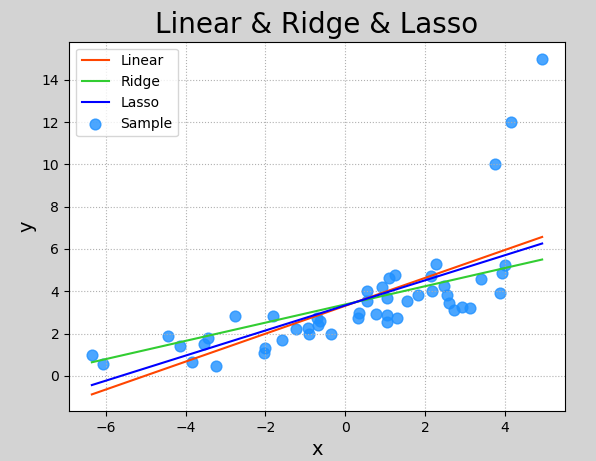
Logically, both Lasso regression and ridge regression can be understood as reducing the coefficient of the function by adjusting the loss function, so as to avoid over fitting to the sample and reduce the weight of the sample with large deviation and its influence on the model

The following is about the sklearn implementation of Lasso regression in ridge regression:

# Lasso regression and ridge regression examples
import numpy as np
# linear model
import sklearn.linear_model as lm
# Model performance evaluation module
import sklearn.metrics as sm
import matplotlib.pyplot as mp

x, y = [], []  # Input and output samples
with open("abnormal.txt", "rt") as f:
    for line in f.readlines():
        data = [float(substr) for substr in line.split(",")]
        x.append(data[:-1])
        y.append(data[-1])

x = np.array(x)  # Input matrix in the form of two-dimensional data, with one sample per row and one feature per column
y = np.array(y)  # An output sequence in the form of a one-dimensional array. Each element corresponds to an input sample
# print(x)
# print(y)

# Create linear regressor
model = lm.LinearRegression()
# Training regressors with known input and output data sets
model.fit(x, y)
# Predict the output according to the training model
pred_y = model.predict(x)

# Create and train ridge regressors
# Ridge: the first parameter is regular intensity. The larger the value, the smaller the weight of abnormal samples
model_2 = lm.Ridge(alpha=200, max_iter=1000)  # Creating objects, max_iter is the maximum number of iterations
model_2.fit(x, y)  # train
pred_y2 = model_2.predict(x)  # forecast

# lasso regression
model_3 = lm.Lasso(alpha=0.5,  # Coefficient of L1 norm multiplication
                   max_iter=1000)  # Maximum number of iterations
model_3.fit(x, y)  # train
pred_y3 = model_3.predict(x)  # forecast

# Visual regression curve
mp.figure('Linear & Ridge & Lasso', facecolor='lightgray')
mp.title('Linear & Ridge & Lasso', fontsize=20)
mp.xlabel('x', fontsize=14)
mp.ylabel('y', fontsize=14)
mp.tick_params(labelsize=10)
mp.grid(linestyle=':')
mp.scatter(x, y, c='dodgerblue', alpha=0.8, s=60, label='Sample')
sorted_idx = x.T[0].argsort()

mp.plot(x[sorted_idx], pred_y[sorted_idx], c='orangered', label='Linear')  # linear regression
mp.plot(x[sorted_idx], pred_y2[sorted_idx], c='limegreen', label='Ridge')  # Ridge regression
mp.plot(x[sorted_idx], pred_y3[sorted_idx], c='blue', label='Lasso')  # Lasso regression

mp.legend()
mp.show()

The following are the results of the implementation:

Model saving and loading

You can save model objects using the functions provided by Python The usage is as follows:

import pickle
# Save model
pickle.dump(Model object, File object)   
# Loading model
model_obj = pickle.load(File object)

Save the training model after the training or evaluation is completed. The complete code is as follows:

# Model save example
import numpy as np
import sklearn.linear_model as lm # linear model
import pickle

x = np.array([[0.5], [0.6], [0.8], [1.1], [1.4]])  # Input set
y = np.array([5.0, 5.5, 6.0, 6.8, 7.0])  # Output set

# Create linear regressor
model = lm.LinearRegression()
# Training regressors with known input and output data sets
model.fit(x, y)

print("Training complete.")

# Save the trained model
with open('linear_model.pkl', 'wb') as f:
    pickle.dump(model, f)
    print("Save model complete.")

After the execution, you can see that there is an additional directory named linear in the same directory as the source code_ model. Pkl file, which is the saved training model Use this model code:

# Model loading example
import numpy as np
import sklearn.linear_model as lm  # linear model
import sklearn.metrics as sm  # Model performance evaluation module
import matplotlib.pyplot as mp
import pickle

x = np.array([[0.5], [0.6], [0.8], [1.1], [1.4]])  # Input set
y = np.array([5.0, 5.5, 6.0, 6.8, 7.0])  # Output set

# Loading model
with open('linear_model.pkl', 'rb') as f:
    model = pickle.load(f)
    print("Loading model complete.")

# Predict the output according to the loaded model
pred_y = model.predict(x)

# Visual regression curve
mp.figure('Linear Regression', facecolor='lightgray')
mp.title('Linear Regression', fontsize=20)
mp.xlabel('x', fontsize=14)
mp.ylabel('y', fontsize=14)
mp.tick_params(labelsize=10)
mp.grid(linestyle=':')
mp.scatter(x, y, c='blue', alpha=0.8, s=60, label='Sample')

mp.plot(x, pred_y, c='orangered', label='Regression')

mp.legend()
mp.show()

The execution result is the same as that predicted by the training model

Linear regression summary

(1) What is linear model: linear model is one of the simplest models in nature, which reflects the proportional growth relationship between independent variables and dependent variables

(2) When to use linear regression: linear models can only be used in data that meet the law of linear distribution

(3) How to realize linear regression: given a set of samples, given the initial w and b, find the optimal w and b by gradient descent method