Basic concepts

What is support vector machine

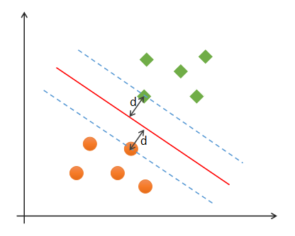
Support Vector Machines is a binary classification model, which is widely used in machine learning, computer vision and data mining. It is mainly used to solve the problem of data classification. Its purpose is to find a hyperplane to segment the samples. The principle of segmentation is to maximize the interval (that is, the distance d from the edge point of the data set to the dividing line is the largest, as shown in the figure below), Finally, it is transformed into a convex quadratic programming problem. Usually SVM is used for binary classification problems. For multivariate classification, it can be decomposed into multiple binary classification problems and then classified. The so-called "support vector" is the edge point crossed by the dotted line in the figure below. The support vector machine corresponds to the line that can correctly divide the data and has the largest interval (the red line in the figure below).

Optimal classification boundary

What is the optimal classification boundary? Under what conditions is the classification boundary the optimal boundary?

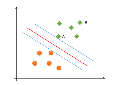
As for the two sample points a and B in the figure, the degree of certainty that point B is predicted to be a positive class is greater than that of point A. therefore, the goal of SVM is to find a hyperplane so that there can be a greater interval between heterogeneous points close to the hyperplane, that is, it is not necessary to consider all sample points, but to maximize the interval between points close to it. The hyperplane can be described by the following linear equation:

w^T x + b = 0

Where, x=(x_1;x_2;...;x_n), w=(w_1;w_2;...;w_n), b is the offset term It can be mathematically proved that the distance from the support vector to the hyperplane is:

\gamma = \frac{1}{||w||}

To maximize the distance, just minimize | w 𞓜

Optimal boundary requirements of SVM

When finding the optimal boundary, SVM needs to meet the following requirements:

(1) Correctness: most samples can be classified correctly;

(2) Security: support vector, that is, the farthest distance between samples closest to the classification boundary;

(3) Fairness: the distance between support vector and classification boundary is equal;

(4) Simplicity: linear equation (line, plane) is used to represent the classification boundary, also known as segmentation hyperplane. If you can't find a higher dimension in the original space by linear transformation, you can't find a higher dimension in the original space The transformation from low latitude space to high latitude space is carried out by kernel function.

Linearly separable and linearly nonseparable

① Linearly separable

If a group of samples can use a linear function to correctly classify the samples, these data samples are said to be linearly separable. So what is a linear function? It is a straight line in two-dimensional space and a plane in three-dimensional space. By analogy, if the spatial dimension is not considered, such linear functions are collectively referred to as hyperplanes.

② Linear inseparable

If a group of samples cannot find a linear function to correctly classify the samples, they are said to be linearly indivisible. The following is an example of one-dimensional linear indivisibility:

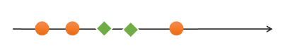
One dimensional linear indivisibility the following is an example of two-dimensional indivisibility:

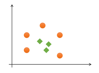
Two dimensional linear indivisibility for this kind of linear indivisibility problem, the low latitude feature space can be mapped to the high latitude feature space by raising the dimension, so as to realize linear indivisibility, as shown in the following figure:

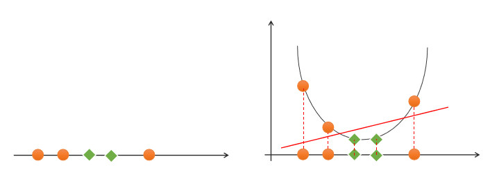
One dimensional space rises to two-dimensional space to realize linear separability! []( https://image.discover304.top/ai/svm_6.png )From two-dimensional space to three-dimensional space to realize linear separability, so how to realize dimension upgrading? This requires the use of kernel functions.

kernel function

Through the feature transformation called kernel function, a new feature is added to make the low-dimensional linear separable problem become a high-dimensional linear separable problem. If K(x, y), x, y ∈ exists in low dimensional space Χ， Make K(x, y)= ϕ (x)· ϕ (y) , then K(x, y) is called kernel function, where ϕ (x)· ϕ (y) Is the inner product of X and Y mapped to the feature space, ϕ (x) Is the mapping function of X → H. The following are several commonly used kernel functions.

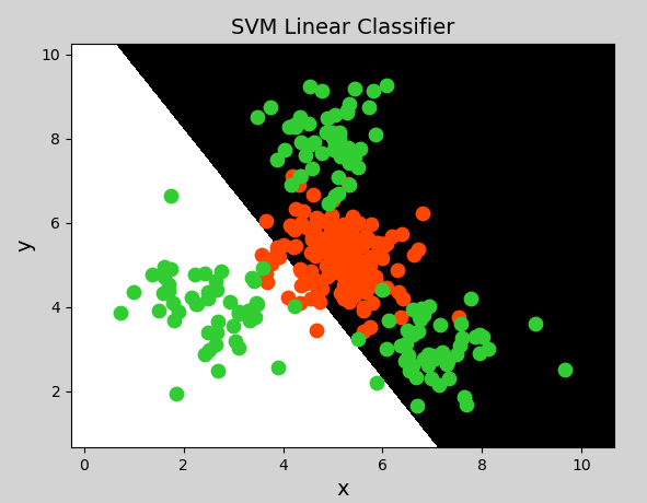
Linear kernel function

Linear kernel function (linear) means that it does not upgrade the dimension through the kernel function, but only seeks the linear classification boundary in the original space. It is mainly used for linear separable problems.

Example code:

# Support vector machine example
import numpy as np
import sklearn.model_selection as ms
import sklearn.svm as svm
import sklearn.metrics as sm
import matplotlib.pyplot as mp

x, y = [], []
with open("../data/multiple2.txt", "r") as f:
    for line in f.readlines():
        data = [float(substr) for substr in line.split(",")]
        x.append(data[:-1])  # input
        y.append(data[-1])  # output

# List to array
x = np.array(x)
y = np.array(y, dtype=int)

# Linear kernel support vector machine classifier
model = svm.SVC(kernel="linear")  # Linear kernel function
# model = svm.SVC(kernel="poly", degree=3)  # Polynomial kernel function
# print("gamma:", model.gamma)
# Radial basis function kernel support vector machine classifier
# model = svm.SVC(kernel="rbf",
#                 gamma=0.01,  # Standard deviation of probability density
#                 C=200)  # Probability intensity
model.fit(x, y)

# Calculate drawing boundaries
l, r, h = x[:, 0].min() - 1, x[:, 0].max() + 1, 0.005
b, t, v = x[:, 1].min() - 1, x[:, 1].max() + 1, 0.005

# Generate grid matrix
grid_x = np.meshgrid(np.arange(l, r, h), np.arange(b, t, v))
flat_x = np.c_[grid_x[0].ravel(), grid_x[1].ravel()]  # merge
flat_y = model.predict(flat_x)  # Classification according to prediction matrix
grid_y = flat_y.reshape(grid_x[0].shape)  # Restore shape

mp.figure("SVM Classifier", facecolor="lightgray")
mp.title("SVM Classifier", fontsize=14)

mp.xlabel("x", fontsize=14)
mp.ylabel("y", fontsize=14)
mp.tick_params(labelsize=10)
mp.pcolormesh(grid_x[0], grid_x[1], grid_y, cmap="gray")

C0, C1 = (y == 0), (y == 1)
mp.scatter(x[C0][:, 0], x[C0][:, 1], c="orangered", s=80)
mp.scatter(x[C1][:, 0], x[C1][:, 1], c="limegreen", s=80)
mp.show()

Draw graphics:

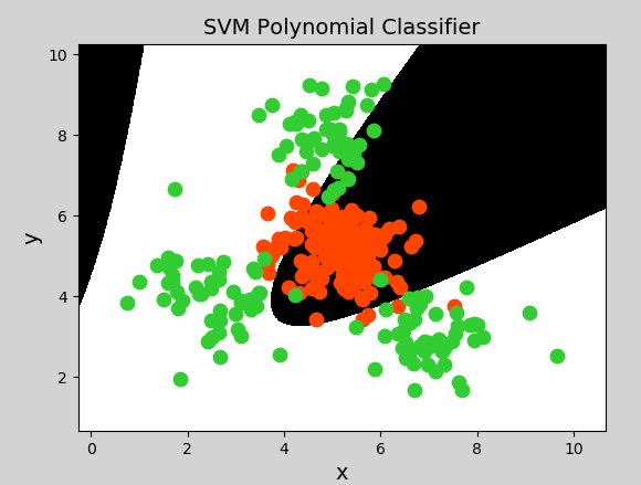
Polynomial kernel function

The Polynomial Kernel uses the method of adding the characteristics of higher-order terms to make dimension raising transformation. When the polynomial order is high, the complexity will be very high. Its expression is:

K(x，y)=(αx^T·y+c)d y = x_1 + x_2\\ y = x_1^2 + 2x_1x_2+x_2^2\\ y=x_1^3 + 3x_1^2x_2 + 3x_1x_2^2 + x_2^3 y=x1​+x2​y=x12​+2x1​x2​+x22​

Among them, α Represents the adjustment parameter, d represents the number of times of the highest order item, and c is an optional constant.

Sample code (just change the support vector machine model created in the previous example to the following code):

model = svm.SVC(kernel="poly", degree=3)  # Polynomial kernel function

Generate image:

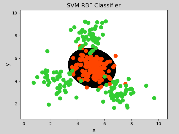
Radial basis kernel function

Radial Basis Function Kernel has strong flexibility and is widely used. Compared with polynomial kernel function, it has fewer parameters, so it has better performance in most cases. When it is uncertain which kernel function to use, the Gaussian kernel function can be verified first. Because it is similar to Gaussian function, it is also called Gaussian kernel function. The expression is as follows:

Sample code (just change the classifier model in the previous example to the following code):

# Radial basis function kernel support vector machine classifier
model = svm.SVC(kernel="rbf",
                gamma=0.01, # Standard deviation of probability density
                C=600)  # Probability intensity, the greater the value, the smaller the tolerance of error classification, the higher the classification accuracy, but the worse the generalization ability; The smaller the value, the greater the tolerance to misclassification, but the stronger the generalization ability

Generate image:

summary

(1) Support vector machine is a binary classification model

(2) Support vector machine finds the optimal linear model as the classification boundary

(3) Boundary requirements: correctness, fairness, security and simplicity

(4) Linear nonseparable problems can be transformed into linear separable problems through kernel functions, including linear kernel function, polynomial kernel function and radial basis kernel function

(5) Support vector machine is suitable for the classification of a small number of samples

Grid search

The way to obtain an optimal super parameter can draw the verification curve, but the verification curve can only obtain one optimal super parameter at a time. If there are many permutations and combinations of multiple hyperparameters, you can use grid search to find the optimal hyperparameter combination.

For each super parameter combination in the super parameter combination list, instantiate the given model, do cv cross validation, and take the super parameter combination with the highest average f1 score as the best choice to instantiate the model object.

Grid search related API s:

import sklearn.model_selection as ms
params = 
[{'kernel':['linear'], 'C':[1, 10, 100, 1000]},
 {'kernel':['poly'], 'C':[1], 'degree':[2, 3]}, 
 {'kernel':['rbf'], 'C':[1,10,100], 'gamma':[1, 0.1, 0.01]}]
 
 
model = ms.GridSearchCV(Model, params, cv=Number of cross validation)
model.fit(Input set)
# Get each parameter combination of grid search
model.cv_results_['params']
# Get the average test score corresponding to each parameter combination of grid search
model.cv_results_['mean_test_score']
# Get the best parameters
model.best_params_
model.best_score_
model.best_estimator_