What is a decision tree

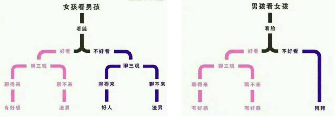
Decision tree is a common machine learning method. Its core idea is that the same (or similar) input produces the same (or similar) output, and the decision is made through the tree structure. Its purpose is to divide the samples with the same attributes into a leaf node through the judgment and decision of different attributes of the samples, so as to realize classification or regression Here are some examples of decision trees in life

[example 1]

Decision tree model of boys looking at girls and girls looking at boys [example 2]

Decision tree model for selecting watermelon in the above example model, through the judgment of a series of characteristics of Watermelon (color, root, knocking, etc.), we finally come to the conclusion: is this a good melon Each decision question raised in the decision-making process is a "test" of an attribute, such as "color =?", "Root =?" The results of each test may be the final conclusion, or the next judgment may be required. The scope of the problem to be considered is within the limit of the last decision result For example, if you judge "root =?" after "color = cyan"

Structure of decision tree

Generally speaking, a decision tree contains a root node, several internal nodes and several leaf nodes The leaf node corresponds to the final decision result, and each other node corresponds to the test of an attribute The samples finally divided into the same leaf node have the same decision attributes. The regression can be realized by averaging the values of these samples, and the classification can be realized by voting on these samples (selecting the category with the largest number of samples)

How to build a decision tree

Constructing decision tree algorithm

The construction of decision tree is to continuously select good features as decision nodes to build a tree structure with strong generalization ability. Its basic algorithm is described as follows:

Obviously, the construction of decision tree is a recursive process, and the core is the following two problems:

• How to select features In each step of decision tree construction, the best features should be selected to make decisions, which has the best effect on data set division;
• Decide when to stop splitting child nodes

How to select features

① Information entropy

information entropy is a common indicator to measure the purity of a sample set. The larger the value, the lower the purity of the set (or the more chaotic). The smaller the value, the higher the purity of the set (or the more orderly) information entropy is defined as follows:

H = -\sum_{i=1}^{n}{P(x_i)log_2P(x_i)}

Where P(x_i) represents the proportion of class I samples in the set. When P(x_i) is 1 (there is only one class, the proportion is 100%), log_ The value of 2P(x_i) is 0, and the information entropy of the whole system is 0; When there are more categories, the value of P(x_i) is closer to 0, log_ When 2P(x_i) approaches negative infinity, the larger the information entropy of the whole system The following code shows the change of the set information entropy of the number of categories from 1... 10:

# Demonstration information entropy calculation
import math
import numpy as np
import matplotlib.pyplot as mp

class_num = 10  # Maximum number of categories


def entropy_calc(n):
    p = 1.0 / n  # Calculate the probability of each category
    entropy_value = 0.0  # Information entropy

    for i in range(n):
        p_i = p * math.log(p)
        entropy_value += p_i

    return -entropy_value  # Return entropy


entropies = []
for i in range(1, class_num + 1):
    entropy = entropy_calc(i)  # Calculate the entropy of category i
    entropies.append(entropy)

print(entropies)

# Visual regression curve
mp.figure('Entropy', facecolor='lightgray')
mp.title('Entropy', fontsize=20)
mp.xlabel('Class Num', fontsize=14)
mp.ylabel('Entropy', fontsize=14)
mp.tick_params(labelsize=10)
mp.grid(linestyle='-')
x = np.arange(0, 10, 1)
print(x)
mp.plot(x, entropies, c='orangered', label='entropy')

mp.legend()
mp.show()

Execution result:

② Information gain

The decision tree judges according to the attributes and divides the samples with the same attributes into the same nodes. At this time, the samples are more orderly (the degree of confusion is reduced) and the value of information entropy is reduced. Subtracting the information entropy after division from the information entropy before division is the information gain obtained by the decision tree. It can be expressed by the following expression:

Gain(D, a) = Ent(D) - \sum_{v=1}^{V} \frac{|D^v|}{|D|} Ent(D^v)

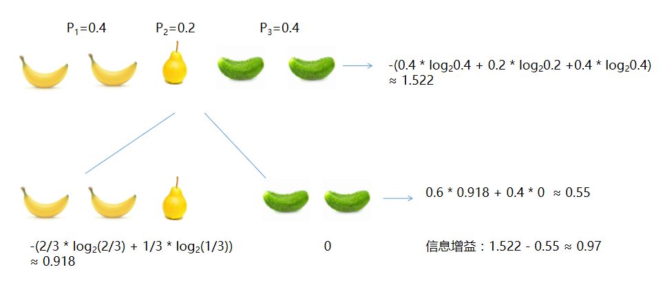
Where, D represents the sample set, a represents the attribute, v represents the possible value of the attribute {v ^ 1, v ^ 2,..., v ^ n}, \ frac {d ^ v} {D} represents the weight. More branches with more samples have a greater impact on the classification results and give higher weight. Gain(D,a) represents the information gain obtained by dividing sub nodes with attribute a on sample set D The following is an example of information gain calculation

explain:

• Bananas account for 2 / 5, so P_1=0.4； Pears account for 1 / 5, so P_2 = 0.2； Cucumber accounts for 1 / 5, so P_3 = 0.4
• Root node information entropy: - (0.4 * log_2 0.4 + 0.2 * log_2 0.2 + 0.4 * log_2 0.4) \approx 1.522
• Divided by color: Yellow Branch Information Entropy - (\ frac{2}{3} * log_2 \frac{2}{3} + \frac{1}{3} * log_2 \frac{1}{3}) \approx 0.918; Green branch information entropy - (1.0 * log_2 1.0) = 0; The information entropy of the whole second layer is 0.6 * 0.918 + 0.4 * 0 \approx 0.55
• Information gain after color division: 1.522 - 0.55 \approx 0.97

It can be seen from the above example that after classifying the samples according to color, the information entropy after division is lower than the original, and the value of decline is the information gain. Generally speaking, the greater the information gain, the greater the "purity improvement" obtained by dividing by this attribute The famous ID3 decision tree learning algorithm divides attributes based on information gain

③ Gain rate

The gain rate does not directly use the information gain, but the ratio of information gain to entropy is used as the standard to measure the quality of features C4. The algorithm uses the gain rate as the standard to divide the attributes Gain rate is defined as:

Gain\_ratio(D, a) = \frac{Gain(D, a)}{IV(a)}

among

IV(a) = - \sum_{v=1}^{V} \frac{|D^v|}{|D|} log_2 \frac{|D^v|}{|D|}

④ Gini coefficient

Gini coefficient is defined as:

Gini(p) = \sum_{k=1}^{k} p_k (1-p_k) = 1 - \sum_{k=1}^{k} p_k^2

Intuitively, Gini coefficient reflects the probability that two samples are randomly selected from data set D and the category marks are inconsistent Therefore, the smaller the Gini coefficient, the higher the purity of the data set CART decision tree uses Gini coefficient to select partition attributes. When selecting attributes, select the attribute with the lowest Gini value after partition as the optimal attribute Using the same symbol as the above formula, the Gini coefficient of attribute a under dataset D is defined as:

Gini\_index(D, a) = \sum_{v=1}^{V} \frac{|D^v|}{|D|} Gini(D^v)

How to stop Division

The following situations will stop the construction of sub nodes of the decision tree:

• All samples in the current node belong to the same category and do not need to be divided
• The current attribute set is empty, or all samples have the same value, so it cannot be divided
• The sample set contained in the current node is empty and cannot be divided
• The number of current node samples is less than the specified number

How to implement decision tree

API related to decision tree in scikit learn:

# Model
model = st.DecisionTreeRegressor(max_depth=4)  # Decision tree regressor
# train
model.fit(train_x, train_y)
# forecast
pre_test_y = model.predict(test_x)

[case] Boston house price forecast

• Data set introduction The data set is an open house price data set, including 506 samples, each of which contains 13 features and 1 label, as shown below:

• code implementation

# Decision tree regression example
# Predicting Boston house prices using decision trees

import sklearn.datasets as sd
import sklearn.utils as su
import sklearn.tree as st
import sklearn.ensemble as se
import sklearn.metrics as sm


boston = sd.load_boston()  # Load boston area house price data
print(boston.feature_names)
print(boston.data.shape)
print(boston.target.shape)

random_seed = 7  # Random seed, calculate the random value, and the same random seed will get the same random value
x, y = su.shuffle(boston.data, boston.target, random_state = random_seed)
# Calculate the number of training data
train_size = int(len(x) * 0.8) # In. Boston 80% of the data in data is used as training data
# Build training data and test data
train_x = x[:train_size]  # Training input, x the first 80% of the data
test_x = x[train_size:]   # Test input, x the next 20% of the data
train_y = y[:train_size]  # Training output
test_y = y[train_size:]   # Test output

######## Single tree prediction ########
# Model
model = st.DecisionTreeRegressor(max_depth=4)  # Decision regressor

# train
model.fit(train_x, train_y)
# forecast
pre_test_y = model.predict(test_x)
# Print R2 value of predicted output and actual output
print(sm.r2_score(test_y, pre_test_y))

• results of enforcement

['CRIM' 'ZN' 'INDUS' 'CHAS' 'NOX' 'RM' 'AGE' 'DIS' 'RAD' 'TAX' 'PTRATIO'
 'B' 'LSTAT']
(506, 13)
(506,)
0.8202560889408634

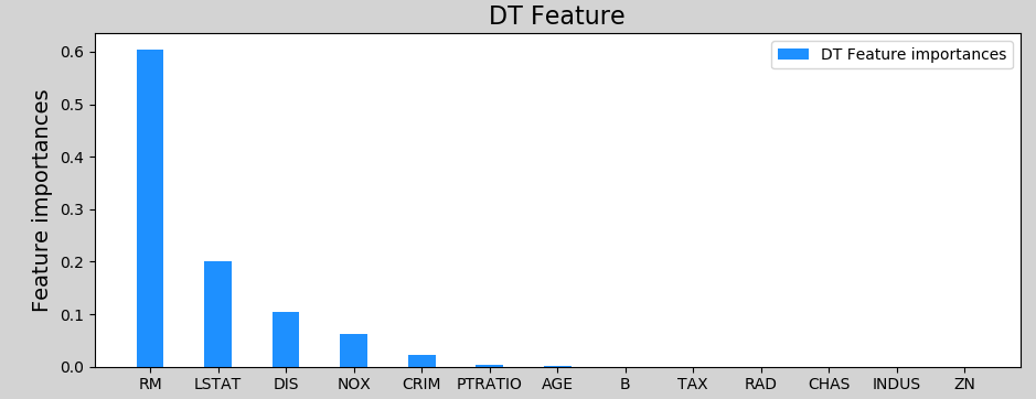
• Characteristic importance

As a by-product in the training process of decision tree model, the reduction of information entropy before and after each feature is divided into sub tables indicates the importance of the feature, which is the index of the importance of the feature. The model object obtained after training provides attribute features_ importances_ To store the importance of each feature. In engineering application, the decision tree can be optimized. Instead of allowing each feature to participate in sub table division, only the more important (or influential) features can be selected as the basis for sub table division. The evaluation index of feature importance is the amount of information entropy reduction brought by dividing the sub table according to the feature. The greater the entropy reduction, the more important it is, and the more priority it takes to participate in the division of the sub table.

Add the following code to the above example:

import matplotlib.pyplot as mp
import numpy as np
fi = model.feature_importances_  # Get feature importance
print("fi:", fi)

# Feature importance visualization
mp.figure("Feature importances", facecolor="lightgray")
mp.plot()
mp.title("DT Feature", fontsize=16)
mp.ylabel("Feature importances", fontsize=14)
mp.grid(linestyle=":", axis=1)
x = np.arange(fi.size)
sorted_idx = fi.argsort()[::-1]  # Importance ranking (reverse order)
fi = fi[sorted_idx]  # Rearrange characteristic values according to sorting index
mp.xticks(x, boston.feature_names[sorted_idx])
mp.bar(x, fi, 0.4, color="dodgerblue", label="DT Feature importances")

mp.legend()
mp.tight_layout()
mp.show()

Execution result:

Pruning of decision tree

pruning is the main method of decision tree learning algorithm to deal with "over fitting" In decision tree learning, in order to correctly classify training samples as much as possible, the node division process will continue to repeat, sometimes resulting in too many branches of the decision tree. At this time, it may be too good to take some characteristics of the training set itself as the general properties of the data Therefore, the risk of overfitting can be reduced by actively removing some branches

(1) Pre pruning In the process of decision tree generation, each node is evaluated before division. If the current node cannot improve the generalization performance of decision tree, the division is stopped and the current node is marked as leaf node

(2) Back pruning Firstly, it is trained as a complete decision tree, and then the non leaf node is investigated from low to top. If replacing the subtree corresponding to the node with leaf node can improve the generalization ability of the decision tree, the subtree is replaced with leaf node

Ensemble learning and random forest

Integrated learning

Ensemble learning completes the learning task by constructing and merging multiple models, so as to obtain significantly superior generalization performance than a single learning model. In short, ensemble learning is to use the "collective wisdom" of the model to improve the accuracy of prediction According to the way of single model, integrated learning can be divided into two categories:

• There is a strong dependency between individuals and the serialization method must be generated serially, which is represented by the Boosting algorithm;
• There is no strong dependence between individuals, and the parallelization methods that can be generated at the same time are Bagging and random forest algorithm

Boosting

What is Boosting

Boosting is a family of algorithms that can promote weak learners to strong learners. Its working principle is:

• First, an initial model is trained;
• Adjust according to the performance of the model to make the data with wrong prediction get more attention, and then retrain the next model;
• Repeat the second step until the number of models reaches the preset number T, and finally combine the T models weighted

AdaBoosting is the most famous algorithm in the Boosting algorithm family. It determines the weight of each sample according to whether the classification of each sample in each training set is correct and the accuracy of the last overall classification. The new data set with modified weights is sent to the lower classifier for training. Finally, the classifiers obtained from each training are fused as the final decision classifier.

Implement Boosting

In sklearn, AdaBoosting related API s:

import sklearn.tree as st
import sklearn.ensemble as se

# Model: decision tree model (single model, base learner)
model = st.DecisionTreeRegressor(max_depth=4)

# n_estimators: build 400 decision trees with different weights and train the model
model = se.AdaBoostRegressor(model, # Single model
                             n_estimators=400, # Number of decision trees
                             random_state=7)# Random seed

# Training model
model.fit(train_x, train_y)

# test model 
pred_test_y = model.predict(test_x)

code:

# AdaBoosting example
# Using AdaBoosting to forecast house prices in Boston
import sklearn.datasets as sd
import sklearn.utils as su
import sklearn.tree as st
import sklearn.ensemble as se
import sklearn.metrics as sm

boston = sd.load_boston()  # Load boston area house price data
print(boston.feature_names)
print(boston.data.shape)
print(boston.target.shape)

random_seed = 7  # Random seed, calculate the random value, and the same random seed will get the same random value
x, y = su.shuffle(boston.data, boston.target, random_state = random_seed)
# Calculate the number of training data
train_size = int(len(x) * 0.8) # In. Boston 80% of the data in data is used as training data
# Build training data and test data
train_x = x[:train_size]  # Training input, x the first 80% of the data
test_x = x[train_size:]   # Test input, x the next 20% of the data
train_y = y[:train_size]  # Training output
test_y = y[train_size:]   # Test output

model2 = se.AdaBoostRegressor(st.DecisionTreeRegressor(max_depth=4),
                              n_estimators=400,   # Number of decision trees
                              random_state=random_seed) # Random seed
# train
model2.fit(train_x, train_y)
# forecast
pre_test_y2 = model2.predict(test_x)
# Print R2 value of predicted output and actual output
print(sm.r2_score(test_y, pre_test_y2))

Execution result:

['CRIM' 'ZN' 'INDUS' 'CHAS' 'NOX' 'RM' 'AGE' 'DIS' 'RAD' 'TAX' 'PTRATIO'
 'B' 'LSTAT']
(506, 13)
(506,)
0.9068598725149652

It can be seen that through the AdaBoosting algorithm, the regression model obtains a higher R2 value

Random forest

What is random forest

Random Forest (RF) is an integrated method specially designed for decision tree. It is an extension of Bagging method. It means that each time the decision tree model is constructed, not only some samples are randomly selected, but also some features are randomly selected to construct multiple decision trees This not only avoids the influence of strong samples on the prediction results, but also weakens the influence of strong characteristics, so that the model has stronger generalization ability

Random forest is simple, easy to implement and low computational overhead. It shows strong performance in many real tasks. It is known as "the method representing the level of integrated learning technology"

How to realize random forest

In the forest, API sklearn is random:

import sklearn.ensemble as se

model = se.RandomForestRegressor(
    max_depth, # Maximum depth of decision tree
    n_estimators, # Number of decision trees
    min_samples_split)# If the minimum number of samples in the sub table is less than this number, it will not be split down

The following is the code for Boston house price prediction using random forest:

# Predicting Boston house prices using random forests
import sklearn.datasets as sd
import sklearn.utils as su
import sklearn.tree as st
import sklearn.ensemble as se
import sklearn.metrics as sm

boston = sd.load_boston()  # Load boston area house price data
print(boston.feature_names)
print(boston.data.shape)
print(boston.target.shape)

random_seed = 7  # Random seed, calculate the random value, and the same random seed will get the same random value
x, y = su.shuffle(boston.data, boston.target, random_state=random_seed)
# Calculate the number of training data
train_size = int(len(x) * 0.8)  # In. Boston 80% of the data in data is used as training data
# Build training data and test data
train_x = x[:train_size]  # Training input, x the first 80% of the data
test_x = x[train_size:]  # Test input, x the next 20% of the data
train_y = y[:train_size]  # Training output
test_y = y[train_size:]  # Test output

# Create a random forest regressor and train it
model = se.RandomForestRegressor(max_depth=10,  # Maximum depth
                                 n_estimators=1000,  # Number of trees
                                 min_samples_split=2)  # The minimum number of samples. If it is less than this number, no child nodes will be divided
model.fit(train_x, train_y)  # train

# Characteristic importance based on day statistics
fi_dy = model.feature_importances_
# print(fi_dy)
pre_test_y = model.predict(test_x)
print(sm.r2_score(test_y, pre_test_y))  # Print r2 score

Printout:

['CRIM' 'ZN' 'INDUS' 'CHAS' 'NOX' 'RM' 'AGE' 'DIS' 'RAD' 'TAX' 'PTRATIO'
 'B' 'LSTAT']
(506, 13)
(506,)
0.9271955403309159

summary

1) What is a decision tree: use the sample characteristics to make decision classification, and divide the samples with the same attributes into a child node

2) Purpose of decision tree: used as classifier and regressor

3) How to build a decision tree: it is built according to information gain, gain rate and Gini coefficient

4) When to use decision tree: it is widely practical, and the course is used for general regression and classification problems

5) Decision tree optimization: ensemble learning, random forest