catalogue
Summary of naive Bayesian algorithm
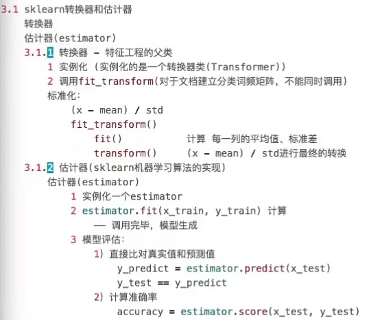
1, Converter and estimator
2, Classification algorithm
K-nearest neighbor algorithm
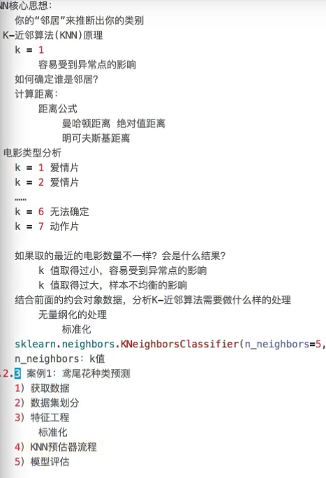
KNN algorithm summary:
advantage:
Simple, easy to understand, easy to implement, no training
Disadvantages:
1) the K value must be specified. If the K value is not selected properly, the classification accuracy cannot be guaranteed.
2) lazy algorithm, which has a large amount of calculation and memory overhead when classifying test samples
Usage scenario:
For small data scenarios, there are thousands to tens of thousands of samples. The specific use depends on the business scenario.
Case code:
from sklearn.datasets import load_iris
from sklearn.model_selection import train_test_split
from sklearn.preprocessing import StandardScaler
from sklearn.neighbors import KNeighborsClassifier


def knn_iris():
    """
    use KNN Algorithm pair iris Data classification
    :return:
    """
    # 1) Get data
    iris = load_iris()

    # 2) Partition dataset
    x_train, x_test, y_train, y_test = train_test_split(iris.data, iris.target, random_state=6
                                                        )
    # 3) Feature Engineering: Standardization
    transfer = StandardScaler()
    x_train = transfer.fit_transform(x_train)
    x_test = transfer.transform(x_test)

    # 4) KNN algorithm predictor
    estimator = KNeighborsClassifier(n_neighbors=3)
    estimator.fit(x_train, y_train)

    # 5) Model evaluation
    # Method 1: directly compare the real value with the predicted value
    y_predict = estimator.predict(x_test)
    print("y_predict:\n", y_predict)
    print("Direct comparison between real value and predicted value:\n", y_test == y_predict)

    # Method 2: calculation accuracy
    score = estimator.score(x_test, y_test)
    print("The accuracy is:\n", score)

    return None


if __name__ == '__main__':
    # Code 1: classify iris data with KNN algorithm
    knn_iris()
Model selection and tuning
Case code
from sklearn.datasets import load_iris
from sklearn.model_selection import train_test_split
from sklearn.preprocessing import StandardScaler
from sklearn.neighbors import KNeighborsClassifier
from sklearn.model_selection import GridSearchCV
def knn_iris_gscv():
"""
use KNN Algorithm pair iris Data classification,Add grid search and cross validation
:return:
"""
# 1) Get data
iris = load_iris()
# 2) Partition dataset
x_train, x_test, y_train, y_test = train_test_split(iris.data, iris.target, random_state=6
)
# 3) Feature Engineering: Standardization
transfer = StandardScaler()
x_train = transfer.fit_transform(x_train)
x_test = transfer.transform(x_test)
# 4) KNN algorithm predictor
estimator = KNeighborsClassifier()
# Join grid search and cross validation
# Parameter preparation
param_dict = {"n_neighbors": [1, 3, 5, 7, 9, 11]}
estimator = GridSearchCV(estimator, param_grid=param_dict, cv=10)
estimator.fit(x_train, y_train)
# 5) Model evaluation
# Method 1: directly compare the real value with the predicted value
y_predict = estimator.predict(x_test)
print("y_predict:\n", y_predict)
print("Direct comparison between real value and predicted value:\n", y_test == y_predict)
# Method 2: calculation accuracy
score = estimator.score(x_test, y_test)
print("The accuracy is:\n", score)
# Best parameter result: best_param_
print("Best parameters:\n", estimator.best_params_)
# Best result: best_score_
print("Best results:\n", estimator.best_score_)
# Best estimator: best_estimator_
print("Best estimator:\n", estimator.best_estimator_)
# Cross validation result: cv_results_
print("Cross validation results:\n", estimator.cv_results_)
return None
if __name__ == '__main__':
# Code 2: classify iris data with KNN algorithm, add grid search and cross validation
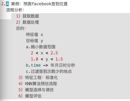
knn_iris_gscv()facebook data mining case:
Case code:
import pandas as pd
from sklearn.model_selection import train_test_split, GridSearchCV
from sklearn.neighbors import KNeighborsClassifier
from sklearn.preprocessing import StandardScaler


def predict_data():
    """
    Data preprocessing
    :return:
    """
    # 1) Read data
    data = pd.read_csv("./train.csv")

    # 2) Basic data processing
    # narrow the range
    data = data.query("x<2.5 & x>2 & y<1.5 & y>1.0")

    # Processing time characteristics
    time_value = pd.to_datatime(data["time"], unit="s")
    date = pd.DatetimeIndex(time_value)
    data.loc[:, "day"] = date.day
    data.loc[:, "weekday"] = date.weekday
    data["hour"] = data.hour

    # 3) Filter locations with less check-in times
    data.groupby("place_id").count()
    place_count = data.groupby("place_id").count()["row_id"]
    data_final = data[data['place_id'].isin(place_count[place_count > 3].index.vlaues)]

    # Filter characteristic value and target value
    x = data_final[["x", "y", "accuracy", "day", "weekday", "hour"]]
    y = data_final["place_id"]

    # Data set partition
    # machine learning
    x_train, x_test, y_train, y_test = train_test_split(x, y)
    # 3) Feature Engineering: Standardization
    transfer = StandardScaler()
    x_train = transfer.fit_transform(x_train)
    x_test = transfer.transform(x_test)

    # 4) KNN algorithm predictor
    estimator = KNeighborsClassifier()

    # Join grid search and cross validation
    # Parameter preparation
    param_dict = {"n_neighbors": [1, 3, 5, 7, 9, 11]}
    estimator = GridSearchCV(estimator, param_grid=param_dict, cv=3)
    estimator.fit(x_train, y_train)

    # 5) Model evaluation
    # Method 1: directly compare the real value with the predicted value
    y_predict = estimator.predict(x_test)
    print("y_predict:\n", y_predict)
    print("Direct comparison between real value and predicted value:\n", y_test == y_predict)

    # Method 2: calculation accuracy
    score = estimator.score(x_test, y_test)
    print("The accuracy is:\n", score)

    # Best parameter result: best_param_
    print("Best parameters:\n", estimator.best_params_)
    # Best result: best_score_
    print("Best results:\n", estimator.best_score_)
    # Best estimator: best_estimator_
    print("Best estimator:\n", estimator.best_estimator_)
    # Cross validation result: cv_results_
    print("Cross validation results:\n", estimator.cv_results_)

    return None


if __name__ == '__main__':
    predict_data()
Naive Bayesian algorithm:
Case code
from sklearn.datasets import load_iris
from sklearn.model_selection import train_test_split
from sklearn.preprocessing import StandardScaler
from sklearn.neighbors import KNeighborsClassifier
from sklearn.model_selection import GridSearchCV
from sklearn.datasets import fetch_20newsgroups
from sklearn.feature_extraction.text import TfidfVectorizer
from sklearn.naive_bayes import MultinomialNB


def nb_news():
    """
    Classification of news with naive Bayesian algorithm
    :return:
    """
    # 1) Get data
    news = fetch_20newsgroups(subset="all")

    # 2) Partition dataset
    x_train, x_test, y_train, y_test = train_test_split(news.data, news.target)

    # 3) Feature engineering text feature extraction tfidf
    transfer = TfidfVectorizer()
    x_train = transfer.fit_transform(x_train)
    x_test = transfer.transform(x_test)

    # 4) Naive Bayesian algorithm predictor flow
    estimator = MultinomialNB()
    estimator.fit(x_train, y_train)

    # 5) Model evaluation
    # Method 1: directly compare the real value with the predicted value
    y_predict = estimator.predict(x_test)
    print("y_predict:\n", y_predict)
    print("Direct comparison between real value and predicted value:\n", y_test == y_predict)

    # Method 2: calculation accuracy
    score = estimator.score(x_test, y_test)
    print("The accuracy is:\n", score)

    return None


if __name__ == '__main__':
    # Code 3: classify news with naive Bayesian algorithm
    nb_news()
Summary of naive Bayesian algorithm
Advantages:
It is not sensitive to missing data, and the algorithm is relatively simple. It is often used in text classification.
High classification accuracy and fast speed.
Disadvantages:
Due to the assumption of sample independence, if the features are related, the prediction effect is not obvious.
Decision tree
Case code:
from sklearn.datasets import load_iris
from sklearn.model_selection import train_test_split
from sklearn.preprocessing import StandardScaler
from sklearn.neighbors import KNeighborsClassifier
from sklearn.model_selection import GridSearchCV
from sklearn.datasets import fetch_20newsgroups
from sklearn.feature_extraction.text import TfidfVectorizer
from sklearn.naive_bayes import MultinomialNB
from sklearn.tree import DecisionTreeClassifier, export_graphviz

def decision_iris():
    """
    Using decision tree pair iris Data classification
    :return:
    """
    # 1) Get dataset
    iris = load_iris()

    # 2) Partition dataset
    x_train, x_test, y_train, y_test = train_test_split(iris.data, iris.target, random_state=22)

    # 3) Decision tree predictor
    estimator = DecisionTreeClassifier(criterion="entropy")
    estimator.fit(x_train, y_train)

    # 4) Model evaluation
    # Method 1: directly compare the real value with the predicted value
    y_predict = estimator.predict(x_test)
    print("y_predict:\n", y_predict)
    print("Direct comparison between real value and predicted value:\n", y_test == y_predict)

    # Method 2: calculation accuracy
    score = estimator.score(x_test, y_test)
    print("The accuracy is:\n", score)

    # Visual decision tree
    export_graphviz(estimator, out_file="iris_tree.dot", feature_names=iris.feature_names)

    return None


if __name__ == '__main__':
    # Code 4: classify iris data with decision tree
    decision_iris()
Decision tree support visualization:
A web page that converts a. dot file to a visual image: Graphviz Online
Decision tree summary:
advantage:
Visualization - highly explanatory
Disadvantages:
It is easy to produce over fitting. At this time, the effect of using random forest will be better
Experimental project of decision tree -- a case of titanic data
Case code:
import pandas as pd
from sklearn.feature_extraction import DictVectorizer
from sklearn.model_selection import train_test_split
from sklearn.tree import DecisionTreeClassifier, export_graphviz


def decision_titanic():
    # 1. Get data
    titanic = pd.read_csv("./titanic.csv")
    print(titanic)

    # Filter characteristic value and target value
    x = titanic[["pclass", "age", "sex"]]
    y = titanic["survived"]

    # 2. Data processing
    # 1) Missing value processing
    x['age'].fillna(x["age"].mean(), inplace=True)

    # 2) Convert to dictionary
    x = x.to_dict(orient="records")

    # 3. Data set partition
    x_train, x_test, y_train, y_test = train_test_split(x, y, random_state=22)

    transfer = DictVectorizer()
    x_train = transfer.fit_transform(x_train)
    x_test = transfer.transform(x_test)

    # 3) Decision tree predictor
    estimator = DecisionTreeClassifier(criterion="entropy", max_depth=8)
    estimator.fit(x_train, y_train)

    # 4) Model evaluation
    # Method 1: directly compare the real value with the predicted value
    y_predict = estimator.predict(x_test)
    print("y_predict:\n", y_predict)
    print("Direct comparison between real value and predicted value:\n", y_test == y_predict)

    # Method 2: calculation accuracy
    score = estimator.score(x_test, y_test)
    print("The accuracy is:\n", score)

    # Visual decision tree
    export_graphviz(estimator, out_file="titanic_tree.dot", feature_names=transfer.get_feature_names())


if __name__ == '__main__':
    decision_titanic()
Use random forest to achieve:
import pandas as pd
from sklearn.feature_extraction import DictVectorizer
from sklearn.model_selection import train_test_split
from sklearn.tree import DecisionTreeClassifier, export_graphviz
from sklearn.ensemble import RandomForestClassifier
from sklearn.model_selection import GridSearchCV


def decision_titanic():
    # 1. Get data
    titanic = pd.read_csv("./titanic.csv")
    print(titanic)

    # Filter characteristic value and target value
    x = titanic[["pclass", "age", "sex"]]
    y = titanic["survived"]

    # 2. Data processing
    # 1) Missing value handling
    x['age'].fillna(x["age"].mean(), inplace=True)

    # 2) Convert to dictionary
    x = x.to_dict(orient="records")

    # 3. Data set partition
    x_train, x_test, y_train, y_test = train_test_split(x, y, random_state=22)

    transfer = DictVectorizer()
    x_train = transfer.fit_transform(x_train)
    x_test = transfer.transform(x_test)

    # 3) Random forest predictor
    estimator = RandomForestClassifier()
    # Join grid search and cross validation
    # Parameter preparation
    param_dict = {"n_estimators": [120, 200, 300, 500, 800, 1200],
                  "max_depth": [5, 8, 15, 25, 30]}
    estimator = GridSearchCV(estimator, param_grid=param_dict, cv=3)
    estimator.fit(x_train, y_train)

    # 4) Model evaluation
    # Method 1: directly compare the real value with the predicted value
    y_predict = estimator.predict(x_test)
    print("y_predict:\n", y_predict)
    print("Direct comparison between real value and predicted value:\n", y_test == y_predict)

    # Method 2: calculation accuracy
    score = estimator.score(x_test, y_test)
    print("The accuracy is:\n", score)

    # Visual decision tree
    export_graphviz(estimator, out_file="titanic_tree.dot", feature_names=transfer.get_feature_names())


if __name__ == '__main__':
    decision_titanic()
Random forest summary
Advantages:
It can run effectively on large data sets
The input samples with high-dimensional features are processed without dimensionality reduction.
summary


Code set of this case:
from sklearn.datasets import load_iris
from sklearn.model_selection import train_test_split
from sklearn.preprocessing import StandardScaler
from sklearn.neighbors import KNeighborsClassifier
from sklearn.model_selection import GridSearchCV
from sklearn.datasets import fetch_20newsgroups
from sklearn.feature_extraction.text import TfidfVectorizer
from sklearn.naive_bayes import MultinomialNB
from sklearn.tree import DecisionTreeClassifier, export_graphviz


def knn_iris():
    """
    use KNN Algorithm pair iris Data classification
    :return:
    """
    # 1) Get data
    iris = load_iris()

    # 2) Partition dataset
    x_train, x_test, y_train, y_test = train_test_split(iris.data, iris.target, random_state=6
                                                        )
    # 3) Feature Engineering: Standardization
    transfer = StandardScaler()
    x_train = transfer.fit_transform(x_train)
    x_test = transfer.transform(x_test)

    # 4) KNN algorithm predictor
    estimator = KNeighborsClassifier(n_neighbors=3)
    estimator.fit(x_train, y_train)

    # 5) Model evaluation
    # Method 1: directly compare the real value with the predicted value
    y_predict = estimator.predict(x_test)
    print("y_predict:\n", y_predict)
    print("Direct comparison between real value and predicted value:\n", y_test == y_predict)

    # Method 2: calculation accuracy
    score = estimator.score(x_test, y_test)
    print("The accuracy is:\n", score)

    return None


def knn_iris_gscv():
    """
    use KNN Algorithm pair iris Data classification,Add grid search and cross validation
    :return:
    """
    # 1) Get data
    iris = load_iris()

    # 2) Partition dataset
    x_train, x_test, y_train, y_test = train_test_split(iris.data, iris.target, random_state=6
                                                        )
    # 3) Feature Engineering: Standardization
    transfer = StandardScaler()
    x_train = transfer.fit_transform(x_train)
    x_test = transfer.transform(x_test)

    # 4) KNN algorithm predictor
    estimator = KNeighborsClassifier()

    # Join grid search and cross validation
    # Parameter preparation
    param_dict = {"n_neighbors": [1, 3, 5, 7, 9, 11]}
    estimator = GridSearchCV(estimator, param_grid=param_dict, cv=10)
    estimator.fit(x_train, y_train)

    # 5) Model evaluation
    # Method 1: directly compare the real value with the predicted value
    y_predict = estimator.predict(x_test)
    print("y_predict:\n", y_predict)
    print("Direct comparison between real value and predicted value:\n", y_test == y_predict)

    # Method 2: calculation accuracy
    score = estimator.score(x_test, y_test)
    print("The accuracy is:\n", score)

    # Best parameter result: best_param_
    print("Best parameters:\n", estimator.best_params_)
    # Best result: best_score_
    print("Best results:\n", estimator.best_score_)
    # Best estimator: best_estimator_
    print("Best estimator:\n", estimator.best_estimator_)
    # Cross validation result: cv_results_
    print("Cross validation results:\n", estimator.cv_results_)

    return None


def nb_news():
    """
    Classification of news with naive Bayesian algorithm
    :return:
    """
    # 1) Get data
    news = fetch_20newsgroups(subset="all")

    # 2) Partition dataset
    x_train, x_test, y_train, y_test = train_test_split(news.data, news.target)

    # 3) Feature engineering text feature extraction tfidf
    transfer = TfidfVectorizer()
    x_train = transfer.fit_transform(x_train)
    x_test = transfer.transform(x_test)

    # 4) Naive Bayesian algorithm predictor flow
    estimator = MultinomialNB()
    estimator.fit(x_train, y_train)

    # 5) Model evaluation
    # Method 1: directly compare the real value with the predicted value
    y_predict = estimator.predict(x_test)
    print("y_predict:\n", y_predict)
    print("Direct comparison between real value and predicted value:\n", y_test == y_predict)

    # Method 2: calculation accuracy
    score = estimator.score(x_test, y_test)
    print("The accuracy is:\n", score)

    return None


def decision_iris():
    """
    Using decision tree pair iris Data classification
    :return:
    """
    # 1) Get dataset
    iris = load_iris()

    # 2) Partition dataset
    x_train, x_test, y_train, y_test = train_test_split(iris.data, iris.target, random_state=22)

    # 3) Decision tree predictor
    estimator = DecisionTreeClassifier(criterion="entropy")
    estimator.fit(x_train, y_train)

    # 4) Model evaluation
    # Method 1: directly compare the real value with the predicted value
    y_predict = estimator.predict(x_test)
    print("y_predict:\n", y_predict)
    print("Direct comparison between real value and predicted value:\n", y_test == y_predict)

    # Method 2: calculation accuracy
    score = estimator.score(x_test, y_test)
    print("The accuracy is:\n", score)

    # Visual decision tree
    export_graphviz(estimator, out_file="iris_tree.dot", feature_names=iris.feature_names)

    return None


if __name__ == '__main__':
    # Code 1: classify iris data with KNN algorithm
    # knn_iris()
    # Code 2: classify iris data with KNN algorithm, add grid search and cross validation
    # knn_iris_gscv()
    # Code 3: classify news with naive Bayesian algorithm
    # nb_news()
    # Code 4: classify iris data with decision tree
    decision_iris()