Data consolidation

Common data consolidation methods for pandas:

• pandas.merge connects rows in different DataFrame s based on one or more keys, which is the join operation of the database.
• pandas.concat can stack multiple objects together along an axis
• Instance method combine_first can stitch together duplicate data and fill in missing values from one object with values from another.

pandas.merge

Merge is a database-style merge operation with the following common parameters:

pd.merge(left,right,on='key',how='inner',on='key',left_on='l_key',
				right_on='r_key',left_index=False,right_index=False,
				suffixes=('_left','_right'))

left,right: left and right tables to be merged
how: optional'inner'inner connection,'outer' outer connection,'left'left connection,'right' right connection
on: The key name used for the join must exist in both tables. If not selected, the join key is the intersection of the two tables
left_on, right_on: Not commonly used, left and right tables are used as join keys
left_index,right_index: Use left/right index as join key, default is False
suffixes: used to distinguish common columns, appended to the end of common columns, defaults to ('_x','_y)
join usage is similar to merge but is a Dataframe member method

pandas.concat

concat can connect to Series, defaulting to axis=0 (extended column)

pd.concat(objs,axis=0,join='outer',join_axes=['a','b','c',],keys=['a','b'],
			names=['upper','lower'],ignore_index=True)

Objs is a required parameter, the others are optional parameters, objs input table to join
axis=0 join column
join='outer'/'inner'union or intersection
join_axes specifies an index on another axis, such as axis=1 specifies a row index
keys specify a hierarchical index on the connection axis
ignore_index is not available in both joined table rows and columns

combine_first()

The two arrays may have the same index but different values, so you can't just use merge or concat, where combine_ The first () member method, which applies to both Series and Dataframe, can be seen here as patching the current array with another array

In [115]: df1 = pd.DataFrame({'a': [1., np.nan, 5., np.nan],
   .....:                     'b': [np.nan, 2., np.nan, 6.],
   .....:                     'c': range(2, 18, 4)})

In [116]: df2 = pd.DataFrame({'a': [5., 4., np.nan, 3., 7.],
   .....:                     'b': [np.nan, 3., 4., 6., 8.]})

In [117]: df1
Out[117]: 
     a    b   c
0  1.0  NaN   2
1  NaN  2.0   6
2  5.0  NaN  10
3  NaN  6.0  14

In [118]: df2
Out[118]: 
     a    b
0  5.0  NaN
1  4.0  3.0
2  NaN  4.0
3  3.0  6.0
4  7.0  8.0

In [119]: df1.combine_first(df2)
Out[119]: 
     a    b     c
0  1.0  NaN   2.0
1  4.0  2.0   6.0
2  5.0  4.0  10.0
3  3.0  6.0  14.0
4  7.0  8.0   NaN

Data Aggregation

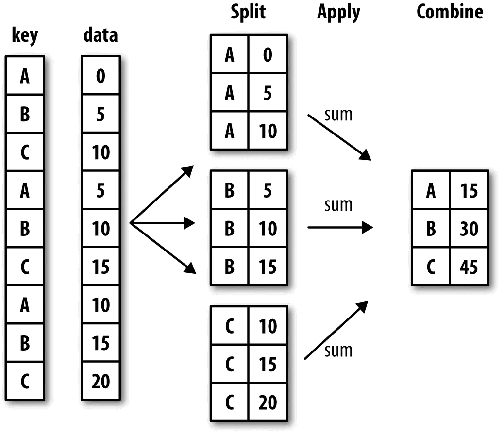
This section uses the groupby function, which is similar to the grouping query mechanism in databases, and has similar functions in pandas.

First split into groups based on the keys provided, then aggregate
Only one attribute aggregation can be selected after grouping

b=df.groupby('Sex')[['Fare']].mean()
b

			Fare
Sex	
female	44.479818
male	25.523893

The same functionality can be written as follows:

a=df['Survived'].groupby(df['Sex']).value_counts()
a

Sex     Survived
female  1           233
        0            81
male    0           468
        1           109
Name: Survived, dtype: int64

agg() function can also be applied

df.groupby('Sex')['Fare'].agg(['mean','count'])

Custom functions can also be passed in:

In [54]: def peak_to_peak(arr):
   ....:     return arr.max() - arr.min()
In [55]: grouped.agg(peak_to_peak)
Out[55]: 
         data1     data2
key1                    
a     2.170488  1.300498
b     0.036292  0.487276

However, incoming customizations can be much slower than the built-in optimized functions because of the overhead (function calls, data rearrangements, and so on) of constructing intermediate grouped data blocks.