Some records and summary of learning modeling in the past six months
1, Linear region
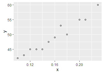
For such a data with obvious linear trend, we should find a straight line to make it have the ability to predict the trend of the data, and adopt the least square estimates, that is, the fitted straight line conforms to the criterion of minimizing the sum of squares of residuals. The following model can be obtained by translating the above into mathematical language
This is a convex optimization problem. We can use the method of advanced mathematics to substitute the constraints into the objective function to obtain an unconstrained optimization, and then calculate the partial derivatives of a and b respectively to obtain the estimates of a and b. statistically, it can be proved that LSE obtains the unbiased estimates of parameters a and b, i.e
In addition, the estimation of parameters a and b can also be obtained by maximum likelihood estimation, and the result is the same as LSE.
Sum of squares of total deviations: SST

Sum of squares of regression: SSR

Sum of squares of residuals: SSE
It can be proved that the sum of three squares satisfies
According to the least square criterion, for different models, the sum of squares of residuals of different models can be compared to select the model with the best fitting ability
Define goodness of fit The smaller the SSE, the greater the value, but it will not exceed 1.
Supply: in machine learning, the error of the model is divided into training error and generalization error. The R side here can only reflect the training error of the model, and a small training error does not necessarily mean that the model has excellent prediction ability, that is, a small training error does not mean a small generalization error. When the model is over fitted, we think it does not have the ability to predict data. For details, refer to Li Hang's statistical machine learning, which will not be described in detail in this paper. When performing polynomial regression on two-dimensional data, the polynomial degree used is too high, which often leads to over fitting (which can be imagined as the extreme case of interpolation).
2, Visualization of + ggplot in R language
lm function can be used not only for univariate linear fitting, but also for multivariate linear and nonlinear fitting.
##Input dataset
x <- c(0.1, 0.11 ,0.12, 0.13, 0.14, 0.15, 0.16, 0.17, 0.18, 0.20, 0.21, 0.23)
y <- c(42 ,43 ,45 ,45 ,45 ,47.5 ,49 ,53 ,50 ,55 ,55 ,60)
##Create data frame
linear <- data.frame(x,y)
##fitting
model <- lm(y~x,data=linear)
##see
summary(model)

##Output results

Call:
lm(formula = y ~ x, data = linear)

Residuals:
     Min       1Q   Median       3Q      Max
-2.00449 -0.63600 -0.02401  0.71297  2.32451

Coefficients:
            Estimate Std. Error t value Pr(>|t|)
(Intercept)   28.083      1.567   17.92 6.27e-09 ***
x            132.899      9.606   13.84 7.59e-08 ***
---
Signif. codes:  0 '***' 0.001 '**' 0.01 '*' 0.05 '.' 0.1 ' ' 1

Residual standard error: 1.309 on 10 degrees of freedom
Multiple R-squared:  0.9503,    Adjusted R-squared:  0.9454
F-statistic: 191.4 on 1 and 10 DF,  p-value: 7.585e-08
The model gives the estimated value of each parameter. Estimate ^ y = 28.083+132.899x ^ it can be seen that the p-value is very small, so it can be considered that our regression equation is significant
We can use the function confint(model) to get the confidence interval of the model in the range of 2.5% - 97.5%
confint(model)
                2.5 %    97.5 %
(Intercept)  24.59062  31.57455
x           111.49556 154.30337
You can use geom in ggplot_ Smooth function for model visualization
geom_smooth(data,formula,method,se=T,colour,size)
data ~ dataset
formula ~ fitting rule can refer to lm function
Method ~ fitting method {loss: locally weighted regression} lm: linear regression glm: generalized linear regression gam: generalized additive regression
Colour ~ line colour
size ~ line width
se ~ add confidence interval. The default value is True
ggplot(linear,aes(x=x,y=y))+
  geom_point(shape=1,colour="black")+
  ##geom_abline(intercept = 28.083,slope=132.899)
  geom_smooth(method = lm,se = F,colour = "steelblue",size=0.5)+
  theme(plot.title = element_text(hjust=0.5,size=15))+
  labs(title="Linear Regression")+
  theme(panel.grid.major = element_blank(), panel.grid.minor = element_blank(),
panel.border = element_blank(),axis.line =element_line(colour = "black"))+
  annotate("text",x=0.2,y=58,label="y=132.9x+28.08")+
  annotate("text",x=0.2,y=59,parse=TRUE,  label = "atop(R^2==0.9503)",size=4)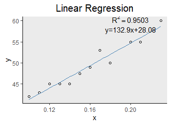
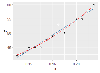
If the formula to be fitted is y=ax^2+b, the following code can be used
x <- c(0.1, 0.11 ,0.12, 0.13, 0.14, 0.15, 0.16, 0.17, 0.18, 0.20, 0.21, 0.23)
y <- c(42 ,43 ,45 ,45 ,45 ,47.5 ,49 ,53 ,50 ,55 ,55 ,60)
##Create data frame
unlinear <- data.frame(x,y)
model <- lm(y~I(x^2),unlinear)
summary(model)


Call:
lm(formula = y ~ I(x^2), data = linear)

Residuals:
     Min       1Q   Median       3Q      Max
-1.46660 -0.59878 -0.07453  0.32904  2.95051

Coefficients:
            Estimate Std. Error t value Pr(>|t|)
(Intercept)  38.3482     0.8144   47.09  4.5e-13 ***
I(x^2)      404.8879    27.5137   14.72  4.2e-08 ***
---
Signif. codes:  0 '***' 0.001 '**' 0.01 '*' 0.05 '.' 0.1 ' ' 1

Residual standard error: 1.234 on 10 degrees of freedom
Multiple R-squared:  0.9559,	Adjusted R-squared:  0.9514
F-statistic: 216.6 on 1 and 10 DF,  p-value: 4.201e-08
It can be seen that the multiple R-squared = 0.9559 at this time is even higher than the 0.9503 of the linear model
y = 38.3482+404.8879x^2
When using lm function for nonlinear fitting, I() must be used in formula
When selecting the model, we should consider not only its training error, but also its generalization ability,
For large sample data, a method is given here, which can take the data to be fitted as non training set and prediction set, use the training set for fitting, and then calculate the sum of squares of residuals of the model on the prediction set, which can be approximately regarded as its generalization error.
In machine learning, a penalty term, regularization, is often added to the error function to prevent overfitting. Its principle is to reduce the parameter variance in the model parameter space (the variance of parameter estimation is often large in overfitting)
The regularization term generally selects the L1 normal form (absolute value) of the parameter vector and the L2 normal form (square sum square) of the parameter vector
The former is called lasso regression and the latter is called ridge regression. For details, please refer to the relevant contents of machine learning, which will not be described in this paper
ps: there's a thing called Occam razor principle. The simpler the model, the better (personal understanding)