1, Overview

1. Three layer api of Matplotlib

The principle or basic logic of matplotlib is to render graphics on the canvas with Artist objects.
It is similar to the steps of human painting:

1. Prepare a canvas or drawing paper
2. Prepare paint, brush and other drawing tools
3. paint a picture

Therefore, matplotlib has three levels of API s:

matplotlib. backend_ bases. Figure canvas represents the drawing area. All images are completed in the drawing area
matplotlib.backend_bases.Renderer represents a renderer, which can be roughly understood as a brush, and controls how to draw on figure canvas.
matplotlib.artist.Artist represents a specific chart component, that is, it calls the Renderer interface to draw on Canvas.
The first two deal with the bottom interaction between the program and the computer. The third artist is to call the interface to make the diagram we want, such as the setting of graphics, text and lines. So usually, 95% of our time is spent with Matplotlib artist. Artist class.

2. Classification of artist

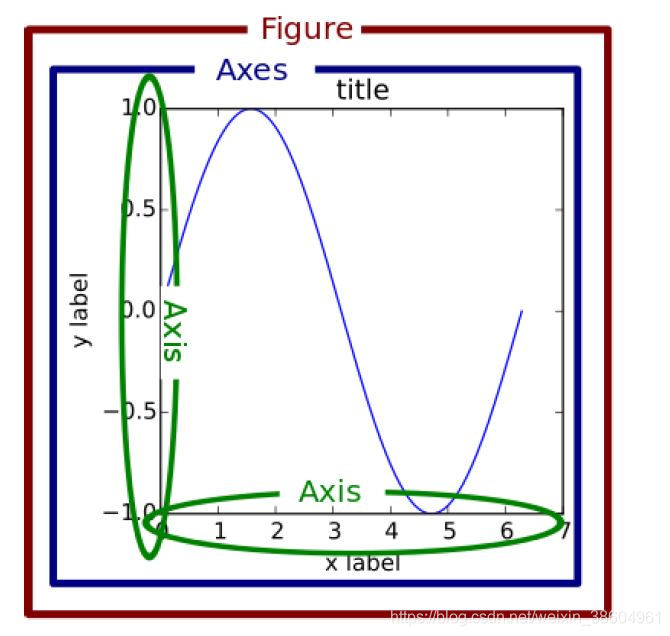
There are two types of artists: primitives and containers.

primitive is a basic element. It contains some standard graphic objects we want to use in drawing area, such as curve Line2D, text, Rectangle, image, etc.

Container is the container, that is, the place used to hold basic elements, including graphic figure, coordinate system Axes and coordinate Axis. The relationship between them is shown in the figure below:

3. Standard usage of Matplotlib

The standard use process of matplotlib is:

1. Create a Figure instance
2. Use the Figure instance to create one or more Axes or Subplot instances
3. Use the auxiliary methods of the Axes instance to create a primitive

It is worth mentioning that Axes is a container, which is probably the most important class in the matplotlib API, and we spend most of our time dealing with it. More specific information will be described in the container section of section III.

A process example and description are as follows:

import matplotlib.pyplot as plt
import numpy as np

# step 1 
# We use Matplotlib pyplot. Figure () creates an instance of figure
fig = plt.figure()

# step 2
# Then, a drawing area with two rows and one column (that is, there can be two subplots) is created with the Figure instance, and a subplot is created at the first position at the same time
ax = fig.add_subplot(2, 1, 1) # two rows, one column, first plot

# step 3
# Then draw a curve with the method of axe example
t = np.arange(0.0, 1.0, 0.01)
s = np.sin(2*np.pi*t)
line, = ax.plot(t, s, color='blue', lw=2)

2, Basic elements - primitives

Each container may contain a variety of basic elements - primitives, so introduce primitives first, and then containers.

This chapter focuses on several types of primitives: curve Line2D, Rectangle rectangle and image (Text text is complex and will be described in detail later.)

2.1 2DLines

In matplotlib, the curve is drawn mainly through the class matplotlib lines. Line2d.
Its base class: Matplotlib artist. Artist

Meaning of matplotlib midline line line: it can be a solid line style connecting all vertices or a marker for each vertex. In addition, this line will also be affected by the painting style. For example, we can create dotted lines.

Its constructor:

class matplotlib.lines.Line2D(xdata, ydata, linewidth=None, linestyle=None, color=None, marker=None, markersize=None, markeredgewidth=None, markeredgecolor=None, markerfacecolor=None, markerfacecoloralt='none', fillstyle=None, antialiased=None, dash_capstyle=None, solid_capstyle=None, dash_joinstyle=None, solid_joinstyle=None, pickradius=5, drawstyle=None, markevery=None, **kwargs)

The common parameters are:

• xdata: the value of the midpoint of the line to be drawn on the x-axis. If omitted, it defaults to range(1,len(ydata)+1)
• ydata: the value of the midpoint of the line to be drawn on the y-axis
• linewidth: the width of the line
• linestyle: Linetype
• Color: the color of the line
• Marker: marker of points. For details, please refer to the markers API
• size of marker

For other detailed parameters, please refer to the official Line2D documentation

a. How to set the properties of Line2D
There are three ways to set line properties with.

1. Set directly in the plot() function
2. Set the line object by obtaining the line object
3. Get the line attribute and set it with the setp() function

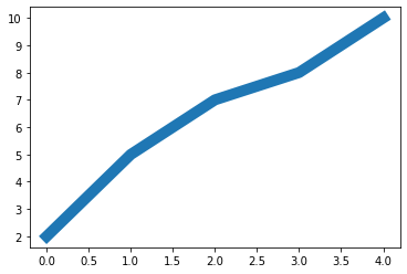
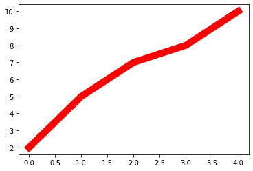
# 1) Set directly in the plot() function
import matplotlib.pyplot as plt
x = range(0,5)
y = [2,5,7,8,10]
plt.plot(x,y, linewidth=10) # Set the line thickness parameter to 10

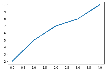
# 2) Set the line object by obtaining the line object
x = range(0,5)
y = [2,5,7,8,10]
line, = plt.plot(x, y, '-')
line.set_antialiased(False) # Turn off anti aliasing

# 3) Get the line attribute and set it with the setp() function
x = range(0,5)
y = [2,5,7,8,10]
lines = plt.plot(x, y)
plt.setp(lines, color='r', linewidth=10)

b. How to draw lines

1. Draw a straight line
2. Error bar drawing error line chart

1) There are two common methods for drawing straight line s:

• pyplot method drawing
• Line2D object painting

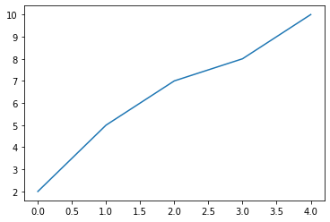
# 1. Plot with pyplot method
import matplotlib.pyplot as plt
x = range(0,5)
y = [2,5,7,8,10]
plt.plot(x,y)

# 2. Line2D object drawing
import matplotlib.pyplot as plt
from matplotlib.lines import Line2D      

fig = plt.figure()
ax = fig.add_subplot(111)
line = Line2D(x, y)
ax.add_line(line)
ax.set_xlim(min(x), max(x))
ax.set_ylim(min(y), max(y))

plt.show()

2) Error bar drawing error line chart
pyplot has a special function for drawing error lines, which is implemented through the errorbar class. Its constructor:

matplotlib.pyplot.errorbar(x, y, yerr=None, xerr=None, fmt='', ecolor=None, elinewidth=None, capsize=None, barsabove=False, lolims=False, uplims=False, xlolims=False, xuplims=False, errorevery=1, capthick=None, *, data=None, **kwargs)

The most important parameters are the first few:

• x: The value of the midpoint of the line to be drawn on the x-axis
• y: The value of the midpoint of the line to be drawn on the y-axis
• yerr: Specifies the y-axis horizontal error
• xerr: Specifies the x-axis horizontal error
• fmt: Specifies the color, shape and line style of a point in the line chart, such as' co – '
• ecolor: Specifies the color of the error bar
• elinewidth: Specifies the line width of the error bar

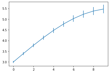
Draw errorbar

fig = plt.figure()
x = np.arange(10)
y = 2.5 * np.sin(x / 20 * np.pi)
yerr = np.linspace(0.05, 0.2, 10)
plt.errorbar(x, y + 3, yerr=yerr, label='both limits (default)')

b. How to draw lines

1. Draw a straight line
2. Error bar drawing error line chart

There are two common methods for drawing straight line s:

x = range(0,5)
y = [2,5,7,8,10]
plt.plot(x,y)

# 2. Line2D object drawing
import matplotlib.pyplot as plt
from matplotlib.lines import Line2D      

fig = plt.figure()
ax = fig.add_subplot(111)
line = Line2D(x, y)
ax.add_line(line)
ax.set_xlim(min(x), max(x))
ax.set_ylim(min(y), max(y))

plt.show()

2) Error bar drawing error line chart
pyplot has a special function for drawing error lines, which is implemented through the errorbar class. Its constructor:

matplotlib.pyplot.errorbar(x, y, yerr=None, xerr=None, fmt='', ecolor=None, elinewidth=None, capsize=None, barsabove=False, lolims=False, uplims=False, xlolims=False, xuplims=False, errorevery=1, capthick=None, *, data=None, **kwargs)

The most important parameters are the first few:

• x: The value of the midpoint of the line to be drawn on the x-axis
• y: The value of the midpoint of the line to be drawn on the y-axis
• yerr: Specifies the y-axis horizontal error
• xerr: Specifies the x-axis horizontal error
• fmt: Specifies the color, shape and line style of a point in the line chart, such as' co – '
• ecolor: Specifies the color of the error bar
• elinewidth: Specifies the line width of the error bar

Draw errorbar

import numpy as np
import matplotlib.pyplot as plt
fig = plt.figure()
x = np.arange(10)
y = 2.5 * np.sin(x / 20 * np.pi)
yerr = np.linspace(0.05, 0.2, 10)
plt.errorbar(x, y + 3, yerr=yerr, label='both limits (default)')

2.2 patches

matplotlib. patches. The patch class is a two-dimensional graphics class. Its base class is Matplotlib artist. Artist, its constructor:

Patch(edgecolor=None, facecolor=None, color=None, linewidth=None, linestyle=None, antialiased=None, hatch=None, fill=True, capstyle=None, joinstyle=None, **kwargs)

a. Rectangle rectangle
The definition of Rectangle class in the official website is: generated by anchor xy and its width and height. The main of Rectangle itself is relatively simple, that is, XY controls the anchor point, and width and height control the width and height respectively. Its constructor:

class matplotlib.patches.Rectangle(xy, width, height, angle=0.0, **kwargs)

In practice, the most common rectangular graphs are hist histogram and bar graph.

1. hist histogram

matplotlib.pyplot.hist(x,bins=None,range=None, density=None, bottom=None, histtype='bar', align='mid', log=False, color=None, label=None, stacked=False, normed=None)

Here are some common parameters:

• x: Data set, the final histogram will make statistics on the data set
• bins: interval distribution of Statistics
• range: tuple, the displayed range. Range takes effect when bins is not given
• density:bool, which is false by default. If it is True, the frequency statistics result will be displayed. Note that the frequency statistics result = number of intervals / (total number * interval width), which is consistent with the normalized effect. density is officially recommended
• histtype: one of {'bar', 'barstacked', 'step', 'stepfilled'} can be selected. The default is bar. It is recommended to use the default configuration. Step uses a ladder shape, and stepfilled will fill the interior of the ladder shape. The effect is similar to that of bar
• align: one of {'left', 'mid' and 'right'} can be selected. The default is' mid ', which controls the horizontal distribution of the histogram. Left or right, there will be some blank areas. It is recommended to use the default
• log: bool, the default is False, that is, whether the index scale is selected for the y coordinate axis
• stacked: bool. The default value is False. Is it a stacked graph

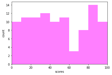
hist draw histogram

import matplotlib.pyplot as plt
import numpy as np 
x=np.random.randint(0,100,100) #Generate 100 data between [0-100], i.e. dataset 
bins=np.arange(0,101,10) #Set continuous boundary values, that is, the distribution interval of histogram [0,10], [10,20) 
plt.hist(x,bins,color='fuchsia',alpha=0.5)#alpha sets the transparency, and 0 is fully transparent 
plt.xlabel('scores') 
plt.ylabel('count') 
plt.xlim(0,100)#Set the x-axis distribution range PLT show()

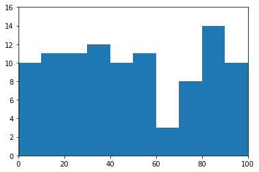
The Rectangle class draws a histogram

import pandas as pd
import re
df = pd.DataFrame(columns = ['data'])
df.loc[:,'data'] = x
df['fenzu'] = pd.cut(df['data'], bins=bins, right = False,include_lowest=True)

df_cnt = df['fenzu'].value_counts().reset_index()
df_cnt.loc[:,'mini'] = df_cnt['index'].astype(str).map(lambda x:re.findall('\[(.*)\,',x)[0]).astype(int)
df_cnt.loc[:,'maxi'] = df_cnt['index'].astype(str).map(lambda x:re.findall('\,(.*)\)',x)[0]).astype(int)
df_cnt.loc[:,'width'] = df_cnt['maxi']- df_cnt['mini']
df_cnt.sort_values('mini',ascending = True,inplace = True)
df_cnt.reset_index(inplace = True,drop = True)

#Draw hist with a Rectangle
import matplotlib.pyplot as plt

fig = plt.figure()
ax1 = fig.add_subplot(111)

for i in df_cnt.index:
    rect =  plt.Rectangle((df_cnt.loc[i,'mini'],0),df_cnt.loc[i,'width'],df_cnt.loc[i,'fenzu'])
    ax1.add_patch(rect)

ax1.set_xlim(0, 100)
ax1.set_ylim(0, 16)
plt.show()

2) bar histogram

matplotlib.pyplot.bar(left, height, alpha=1, width=0.8, color=, edgecolor=, label=, lw=3)

Here are some common parameters:

• left: the position sequence of the x-axis. Generally, the range function is used to generate a sequence, but sometimes it can be a string
• Height: the numerical sequence of the y-axis, that is, the height of the column chart, is generally the data we need to display;
• alpha: transparency. The smaller the value, the more transparent
• Width: refers to the width of the column chart, which is generally 0.8;
• Color or facecolor: the color filled in the column chart;
• edgecolor: shape edge color
• Label: explain the meaning of each image. This parameter paves the way for the legend() function and represents the label of the bar

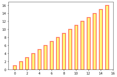
There are two ways to draw a histogram

• bar plot histogram
• The Rectangle class draws a histogram

# bar plot histogram
import matplotlib.pyplot as plt
y = range(1,17)
plt.bar(np.arange(16), y, alpha=0.5, width=0.5, color='yellow', edgecolor='red', label='The First Bar', lw=3)

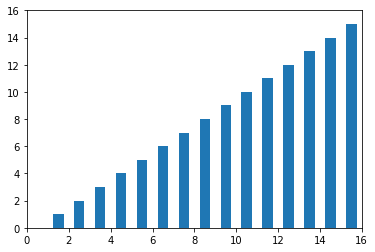
# The Rectangle class draws a histogram
#import matplotlib.pyplot as plt
fig = plt.figure()
ax1 = fig.add_subplot(111)

for i in range(1,17):
    rect =  plt.Rectangle((i+0.25,0),0.5,i)
    ax1.add_patch(rect)
ax1.set_xlim(0, 16)
ax1.set_ylim(0, 16)
plt.show()

b. Polygon polygon
matplotlib. patches. The polygon class is a polygon class. Its base class is Matplotlib patches. Patch, its constructor:

class matplotlib.patches.Polygon(xy, closed=True, **kwargs)

xy is an N × 2, which is the vertex of the polygon.
closed is True to specify that the polygon will coincide with the start and end points, thereby explicitly closing the polygon.

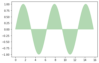
matplotlib. patches. fill class is commonly used in polygon class. It draws a filled polygon based on xy. Its definition:

matplotlib.pyplot.fill(*args, data=None, **kwargs)

Parameter Description: about the sequence of X, y and color, where color is an optional parameter. Each polygon is defined by the X and y position list of its nodes, and a color specifier can be selected later. You can draw multiple polygons by providing multiple x, y, [color] groups.

# Draw graphics with fill
import matplotlib.pyplot as plt
x = np.linspace(0, 5 * np.pi, 1000) 
y1 = np.sin(x)
y2 = np.sin(2 * x) 
plt.fill(x, y1, color = "g", alpha = 0.3)

c. Wedge wedge
matplotlib. patches. The polygon class is a polygon class. Its base class is Matplotlib patches. Patch, its constructor:

class matplotlib.patches.Wedge(center, r, theta1, theta2, width=None, **kwargs)

A Wedge wedge shape is centered on the coordinates x and Y and has a radius r from θ 1 sweep to θ 2 (in degrees).
If the width is given, draw a partial wedge from the inner radius r - width to the outer radius r. Drawing pie chart is common in wedge.

matplotlib.pyplot.pie syntax:

matplotlib.pyplot.pie(x, explode=None, labels=None, colors=None, autopct=None, pctdistance=0.6, shadow=False, labeldistance=1.1, startangle=0, radius=1, counterclock=True, wedgeprops=None, textprops=None, center=0, 0, frame=False, rotatelabels=False, *, normalize=None, data=None)

Make a pie chart of data x, and the area of each wedge is represented by x/sum(x).
The most important parameters are the first four:

• x: Wedge shape, one-dimensional array.
• Expand: if not equal to None, it is a len(x) array that specifies the fraction used to offset the radius of each wedge block.
• labels: used to specify the tag of each wedge block. The value is list or None.
• colors: the color sequence used by the pie chart cycle. If the value is None, the color in the current active loop is used.
• startangle: the drawing angle at the beginning of the pie chart.

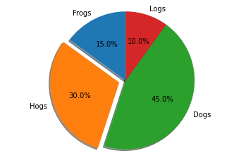
Pie drawing pie chart

import matplotlib.pyplot as plt 
labels = 'Frogs', 'Hogs', 'Dogs', 'Logs'
sizes = [15, 30, 45, 10] 
explode = (0, 0.1, 0, 0) 
fig1, ax1 = plt.subplots() 
ax1.pie(sizes, explode=explode, labels=labels, autopct='%1.1f%%', shadow=True, startangle=90) 
ax1.axis('equal') # Equal aspect ratio ensures that pie is drawn as a circle. 
plt.show()

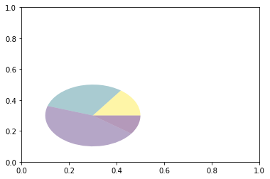
wedge drawing pie chart

import matplotlib.pyplot as plt 
import numpy as np
from matplotlib.patches import Circle, Wedge
from matplotlib.collections import PatchCollection

fig = plt.figure()
ax1 = fig.add_subplot(111)
theta1 = 0
sizes = [15, 30, 45, 10] 
patches = []
patches += [
    Wedge((0.3, 0.3), .2, 0, 54),             # Full circle
    Wedge((0.3, 0.3), .2, 54, 162),  # Full ring
    Wedge((0.3, 0.3), .2, 162, 324),              # Full sector
    Wedge((0.3, 0.3), .2, 324, 360),  # Ring sector
]
colors = 100 * np.random.rand(len(patches))
p = PatchCollection(patches, alpha=0.4)
p.set_array(colors)
ax1.add_collection(p)
plt.show()

c.collections
collections class is used to draw a collection of objects. collections has many different subclasses, such as regularpolycollection, circlecollection and PathCollection, which correspond to different collection subtypes. One of the most commonly used is the scatter graph, which belongs to the subclass of PathCollection. The scatter method provides the encapsulation of this class and draws scatter graphs marked with different sizes or colors according to x and y. Its construction method:

Axes.scatter(self, x, y, s=None, c=None, marker=None, cmap=None, norm=None, vmin=None, vmax=None, alpha=None, linewidths=None, verts=, edgecolors=None, *, plotnonfinite=False, data=None, **kwargs)

The most important parameters are the first five:

• x: Position of data point X axis
• y: Position of the Y-axis of the data point
• s: Size
• c: It can be a string in a single color format or a series of colors
• Marker: type of marker

# Plotting scatter diagram with scatter
x = [0,2,4,6,8,10] 
y = [10]*len(x) 
s = [20*2**n for n in range(len(x))] 
plt.scatter(x,y,s=s) 
plt.show()

d. images
Images is a class for drawing image in matplotlib. The most commonly used imshow can draw images according to the array. Its constructor:

class matplotlib.image.AxesImage(ax, cmap=None, norm=None, interpolation=None, origin=None, extent=None, filternorm=True, filterrad=4.0, resample=False, **kwargs)

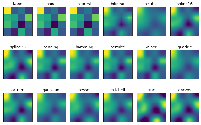
imshow draws an image based on the array

matplotlib.pyplot.imshow(X, cmap=None, norm=None, aspect=None, interpolation=None, alpha=None, vmin=None, vmax=None, origin=None, extent=None, shape=, filternorm=1, filterrad=4.0, imlim=, resample=None, url=None, *, data=None, **kwargs)

When drawing with imshow, you first need to pass in an array. The array corresponds to the pixel position and pixel value in the space. Different difference methods can be set for the interpolation parameter. The specific effects are as follows.

import matplotlib.pyplot as plt
import numpy as np
methods = [None, 'none', 'nearest', 'bilinear', 'bicubic', 'spline16',
           'spline36', 'hanning', 'hamming', 'hermite', 'kaiser', 'quadric',
           'catrom', 'gaussian', 'bessel', 'mitchell', 'sinc', 'lanczos']


grid = np.random.rand(4, 4)

fig, axs = plt.subplots(nrows=3, ncols=6, figsize=(9, 6),
                        subplot_kw={'xticks': [], 'yticks': []})

for ax, interp_method in zip(axs.flat, methods):
    ax.imshow(grid, interpolation=interp_method, cmap='viridis')
    ax.set_title(str(interp_method))

plt.tight_layout()
plt.show()

3, Object container - object container

The container will contain some primitives, and the container has its own properties.
For example, Axes Artist is a container that contains many primitives, such as Line2D and Text; At the same time, it also has its own attributes, such as xscal, to control whether the X-axis is linear or log.

1. Figure container

matplotlib.figure.Figure is the container object container at the top level of Artist, which contains all elements in the diagram. The background of a chart is a rectangular Rectangle in Figure.patch.
When we add figure. Add to the chart_ Subplot () or figure. Add_ When the axes () element, these are added to the Figure.axes list.

fig = plt.figure()
ax1 = fig.add_subplot(211) # Make a 2 * 1 Diagram and select the first sub diagram
ax2 = fig.add_axes([0.1, 0.1, 0.7, 0.3]) # Position parameters, four numbers represent (left,bottom,width,height) respectively
print(ax1) 
print(fig.axes) # fig.axes contains two instances of subplot and axes, which have just been added

Since figure maintains current axes, you should not manually add or delete elements from the Figure.axes list, but through Figure.add_subplot(),Figure.add_axes() to add elements, and Figure.delaxes() to delete elements. However, you can iterate or access the axes in figure. Axes, and then modify the properties of the axes.

For example, the following steps traverse the contents of axes and add grid lines:

fig = plt.figure()
ax1 = fig.add_subplot(211)

for ax in fig.axes:
    ax.grid(True)

Figure also has its own text, line, patch and image. You can add directly through the add primitive statement. However, note that the default coordinate system in figure is in pixels. You may need to convert it to figure coordinate system: (0,0) represents the lower left point and (1,1) represents the upper right point.

Figure common attributes of container:
Figure.patch attribute: the background rectangle of figure
Figure.axes attribute: a list of axes instances (including Subplot)
Figure.images attribute: a list of FigureImages patch
Figure.lines attribute: a list of Line2D instances (rarely used)
Figure.genes attribute: a list of Figure Legend instances (different from axes.genes)
Figure.texts property: a list of text instances

2. Axes container

matplotlib.axes.Axes is the core of Matplotlib. A large number of artists for drawing are stored in it, and it has many auxiliary methods to create and add artists to itself, and it also has many assignment methods to access and modify these artists.

Similar to the Figure container, Axes contains a patch attribute, which is a Rectangle for the Cartesian coordinate system; For polar coordinates, it is a Circle. This patch attribute determines the shape, background, and border of the drawing area.

fig = plt.figure()
ax = fig.add_subplot(111)
rect = ax.patch  # The patch of axes is a Rectangle instance
rect.set_facecolor('green')

Axes has many methods for drawing, such as plot(),. text(),. hist(),. imshow() and other methods are used to create most common primitives (such as Line2D, Rectangle, Text, Image, etc.).

Subplot is a special axis. Its example is a subplot instance located in an area of the grid. In fact, you can also create axes in any area through Figure.add_axes([left,bottom,width,height]) to create axes in any area, where left, bottom, width and height are floating-point numbers between [0-1], which represent coordinates relative to Figure.

You shouldn't go directly through Axes Lines and Axes Use the patches list to add a chart. Because Axes does a lot of automation when creating or adding an object to the diagram:
It will set the attributes of figure and axes in Artist, and default the conversion of axes;
It will also view the data in Artist to update the data structure, so that the data range and rendering mode can be automatically adjusted according to the drawing range.

You can also use the auxiliary method of Axes add_line() and add_patch() method to add directly.

In addition, Axes also contains two most important artist containers:

ax.xaxis: an instance of XAxis object, which is used to handle the drawing of x-axis tick and label
ax.yaxis: an instance of YAxis object, which is used to handle the drawing of y-axis tick and label
It will be described in detail in the following sections.

Common properties of Axes containers are:
artists: Artist instance list patch: rectangle instance where axes is located collections: Collection instance images: Axes image legends: Legend instance lines: Line2D instance patches: Patch instance texts: Text instance xaxis: matchlotlib axis. Xaxis instance yaxis: Matplotlib axis. Yaxis instance

3. Axis container

matplotlib. axis. The axis instance handles the drawing of tick line, grid line, tick label and axis label, including the scale line, scale label, coordinate grid and coordinate axis title on the coordinate axis. Usually, you can configure the left and right scales of the y axis independently, or you can configure the upper and lower scales of the x axis independently.

Scales include major and minor scales, which are Tick scale objects.

Axis also stores data for adaptation, pan, and zoom_ Interval and view_interval. It also has Locator instances and Formatter instances to control the position of tick marks and scale label s.

Each Axis has a label attribute, as well as a list of major and minor scales. These ticks are Axis Xtick and Axis Ytick instances, which contain line primitive and text primitive, are used to render tick marks and scale text.

Scales are created dynamically and only when they need to be created (such as scaling). Axis also provides some auxiliary methods to obtain scale text, tick mark position, etc.:
Common are as follows:

# The results are displayed directly without print
from IPython.core.interactiveshell import InteractiveShell
InteractiveShell.ast_node_interactivity = "all"

fig, ax = plt.subplots()
x = range(0,5)
y = [2,5,7,8,10]
plt.plot(x, y, '-')

axis = ax.xaxis # Axis is the X-axis object
axis.get_ticklocs()     # Get tick mark position
axis.get_ticklabels()   # Get the scale label list (a list of Text instances). You can control whether to output the tick label of minor or major through the minor=True|False keyword parameter.
axis.get_ticklines()    # Gets the list of tick marks (a list of Line2D instances). You can control whether to output the tick line of minor or major through the minor=True|False keyword parameter.
axis.get_data_interval()# Get axis scale interval
axis.get_view_interval()# Gets the interval of the axis viewing angle (position)

The following example shows how to adjust the attributes of some axes and scales (ignoring aesthetics, only for adjustment reference):

fig = plt.figure() # Create a new chart
rect = fig.patch   # Rectangle instance and set it to yellow
rect.set_facecolor('lightgoldenrodyellow')

ax1 = fig.add_axes([0.1, 0.3, 0.4, 0.4]) # Create an axes object, starting from the position of (0.1,0.3), with both width and height of 0.4,
rect = ax1.patch   # The rectangle of ax1 is set to gray
rect.set_facecolor('lightslategray')


for label in ax1.xaxis.get_ticklabels(): 
    # Call the x-axis scale label instance, which is a text instance
    label.set_color('red') # colour
    label.set_rotation(45) # Rotation angle
    label.set_fontsize(16) # font size

for line in ax1.yaxis.get_ticklines():
    # Call the y-axis scale line instance, which is a Line2D instance
    line.set_color('green')    # colour
    line.set_markersize(25)    # marker size
    line.set_markeredgewidth(2)# marker thickness

plt.show()

4. Tick container

matplotlib.axis.Tick is the container object from Figure to Axes to Axis to the end of tick.
Tick includes tick, grid line instance and corresponding label.

All these can be obtained through the tick attribute. The common tick attributes are
Tick.tick1line: Line2D instance
Tick.tick2line: Line2D instance
Tick.gridline: Line2D instance
Tick.label1: Text instance
Tick.label2: Text instance

The y-axis is divided into left and right, so tick 1 corresponds to the left axis; Tick 2 corresponds to the axis on the right.
The x-axis is divided into upper and lower, so tick 1 corresponds to the lower axis; Tick 2 corresponds to the axis on the upper side.

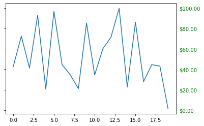
The following example shows how to set the right axis of Y axis as the main axis, and set the label to dollar sign and green:

import numpy as np
import matplotlib.pyplot as plt
import matplotlib

fig, ax = plt.subplots()
ax.plot(100*np.random.rand(20))

# Set the display format of ticker
formatter = matplotlib.ticker.FormatStrFormatter('$%1.2f')
ax.yaxis.set_major_formatter(formatter)

# Set the parameters of ticker. The right side is the spindle and the color is green
ax.yaxis.set_tick_params(which='major', labelcolor='green',
                         labelleft=False, labelright=True)

plt.show()