preface

Matrix decomposition can be used to calculate the predicted value and so on, which is very important, so next I will sort out the process of matrix decomposition and related knowledge.

1, Examples

There is a scoring matrix of R(5,4) as follows: ("-" means that the user does not score)

Where the scoring matrix R(n,m) is n rows and m columns, n represents the number of user s and M rows represents the number of item s

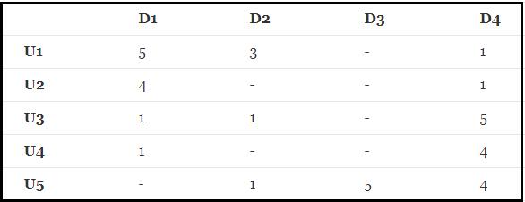
Then, how to predict the score of the non scored goods according to the current matrix R (5,4) (how to get the score of the user with a score of 0)?  

2, Steps

1. Construct Loss function

The loss function is a classical constructor, which is very important.

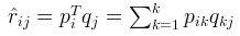
Loss function: use the original scoring matrix

And reconstructed scoring matrix

The square of the error between is taken as the loss function, that is:

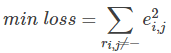
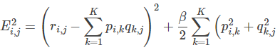
If R(i,j) is known, the sum of squares of errors of R(i,j) is:

Finally, the minimum value of the sum of losses of all non "-" items needs to be solved:

2. Partial derivative

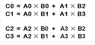
3. Matrix multiplication

Matrix A and matrix B can be multiplied. The number of columns of matrix a must be equal to the number of rows of matrix B

Operation rule: the numbers in each row of A are multiplied by the numbers in each column of B to add up the results

   

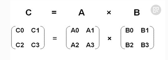
The result of matrix multiplication is the relationship between rows and columns: the number of rows is A and the number of columns is B

2. Because each time it is A row and B column, the outermost two-layer cycle can use the change of the number of rows of A and the number of columns of B

Therefore, for this example:

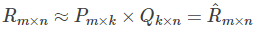
The matrix R can be approximately expressed as the product of P and Q: R (n,m) ≈ P(n,K)*Q(K,m)

In the process of matrix decomposition, the original scoring matrix

Decompose into two matrices

and

Product of:

4. Gradient descent

The minimum loss function is obtained by iterative solution step by step by gradient descent method.

Concepts related to gradient descent:

1. Step size: the step size determines the length of each step along the negative direction of the gradient in the gradient descent iteration process.

2. Feature: refers to the input part of the sample, such as two single feature samples (x0,y0), (x1,y1), then the first sample feature is x0 and the first sample output is y0

3. Hypothesis function: hypothesis function is used to fit the input text

4. Loss function: used to measure the degree of fitting

In this example, the gradient drops:

The modified p and q components are obtained using the gradient descent method:

• Solve the negative gradient of the loss function:

     

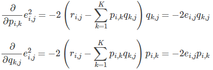
• Update the variable according to the direction of the negative gradient:

     

Keep iterating until the algorithm finally converges (until sum (e ^ 2) < = threshold)

5. Regularization

Adjust the amount of information allowed to be stored by the model, or restrict the information allowed to be stored by the model. If a network can only remember a few patterns, the optimization process will force the model to focus on the most important patterns, which is more likely to be well generalized.

Regularization can be divided into three categories according to strategy

Empirical regularization: lower generalization error methods are realized through engineering skills, such as early termination method, model integration, Dropout, etc;
Parameter regularization: directly provide regularization constraints, such as L1/L2 regularization method;
Implicit regularization: it does not directly provide constraints, such as data related operations, including normalization, data enhancement, disturbing labels, etc.

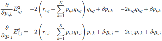
The example is solved by adding the loss function of regularization term:

1. First order

 2. Usually, in the process of solving, in order to have better generalization ability, regular terms will be added to the loss function to constrain the parameters

The regular loss function is:

   

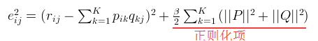
That is:

       

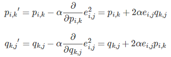
 3. The modified p and q components are obtained using the gradient descent method:

• Solve the negative gradient of the loss function:

        

• Update the variable according to the direction of the negative gradient:

      

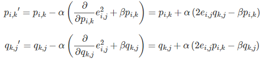
Keep iterating until the algorithm finally converges (until sum (e ^ 2) < = threshold)

[prediction] using the above process, we can get the matrix

and

In this way, you can score the product i ， j ， for the user:

                 

6. The code is as follows:

# !/usr/bin/env python
# encoding: utf-8
__author__ = 'Scarlett'
#Matrix decomposition has been developed and applied in scoring and prediction system
# from pylab import *
import matplotlib.pyplot as plt
from math import pow
import numpy


def matrix_factorization(R,P,Q,K,steps=5000,alpha=0.0002,beta=0.02):
    Q=Q.T  # The. T operation represents the transpose of a matrix
    result=[]
    for step in range(steps):
        for i in range(len(R)):
            for j in range(len(R[i])):
                if R[i][j]>0:
                    eij=R[i][j]-numpy.dot(P[i,:],Q[:,j]) # . dot(P,Q) represents the inner product of the matrix
                    for k in range(K):
                        P[i][k]=P[i][k]+alpha*(2*eij*Q[k][j]-beta*P[i][k])
                        Q[k][j]=Q[k][j]+alpha*(2*eij*P[i][k]-beta*Q[k][j])
        eR=numpy.dot(P,Q)
        e=0
        for i in range(len(R)):
            for j in range(len(R[i])):
                if R[i][j]>0:
                    e=e+pow(R[i][j]-numpy.dot(P[i,:],Q[:,j]),2)
                    for k in range(K):
                        e=e+(beta/2)*(pow(P[i][k],2)+pow(Q[k][j],2))
        result.append(e)
        if e<0.001:
            break
    return P,Q.T,result

if __name__ == '__main__':
    R=[
        [5,3,0,1],
        [4,0,0,1],
        [1,1,0,5],
        [1,0,0,4],
        [0,1,5,4]
    ]

    R=numpy.array(R)

    N=len(R)
    M=len(R[0])
    K=2

    P=numpy.random.rand(N,K) #Randomly generate a matrix with N rows and K columns
    Q=numpy.random.rand(M,K) #Randomly generate a matrix with M rows and K columns

    nP,nQ,result=matrix_factorization(R,P,Q,K)
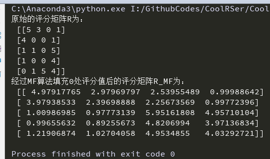
    print("Original scoring matrix R Is:\n",R)
    R_MF=numpy.dot(nP,nQ.T)
    print("after MF The algorithm fills the scoring matrix after 0 scoring values R_MF Is:\n",R_MF)

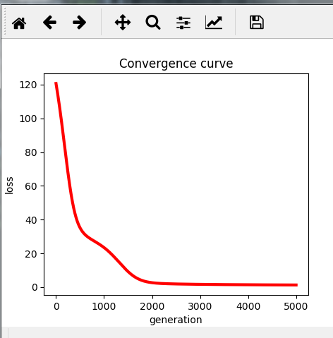
#-------------Convergence curve of loss function---------------

    n=len(result)
    x=range(n)
    plt.plot(x,result,color='r',linewidth=3)
    plt.title("Convergence curve")
    plt.xlabel("generation")
    plt.ylabel("loss")
    plt.show()

Operation results: