AI for medical image analysis
1.Data Exploration course code
In the first assignment of this lesson, you will use the ChestX-ray8 Data were taken from chest X-ray images.
In this notebook, you will have the opportunity to explore this dataset and familiarize yourself with some of the techniques you will use in your first grading assignment
Before you start coding for any machine learning project, the first step is to explore your data. The standard Python package for analyzing and manipulating data is pandas.
Using the next two code cells, you import pandas and a package named numpy for numeric operations, then use pandas to read the csv file into the data frame and print out the first few lines of data.
# Import necessary packages
import pandas as pd
import numpy as np
import matplotlib.pyplot as plt
%matplotlib inline
import os
import seaborn as sns
sns.set()
# Read csv file containing training datadata
train_df = pd.read_csv("nih/train-small.csv")
# Print first 5 rows
print(f'There are {train_df.shape[0]} rows and {train_df.shape[1]} columns in this data frame')
train_df.head()

View the columns in this csv file. This file contains the name of the chest X-ray image ("image" column), and the column filled with 1 and 0 identifies the diagnosis given based on each X-ray image.
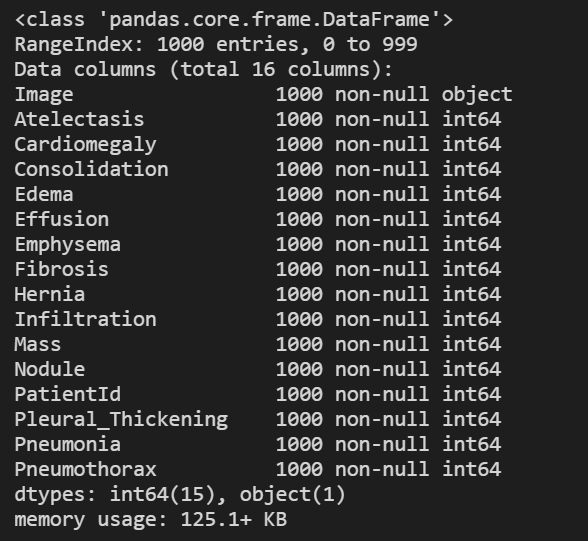
Data type and null check
# Look at the data type of each column and whether null values are present
train_df.info()
Unique ID check
"PatientId" has an identification number for each patient.
One thing you want to know about such medical data sets is whether you are looking at duplicate data for some patients, or whether each image represents a different person.
print(f"The total patient ids are {train_df['PatientId'].count()}, from those the unique ids are {train_df['PatientId'].value_counts().shape[0]} ")
The total patient ids are 1000, from those the unique ids are 928
# pandas value_ The counts() function confirms the frequency of data occurrence
count = train_df['PatientId'].value_counts()
count.shape
count
(928,)

As you can see, the number of unique patients in the dataset is less than the total, so there must be some overlap. For patients with multiple records, you need to ensure that they do not appear in both training and test sets to avoid data leakage (described later in this week's lecture).
Explore data tags
Run the next two code units to create a list of names for each patient condition or disease.
# pandas.keys() returns the column name of pd, which contains different diseases
columns = train_df.keys()
columns = list(columns)
print(columns)

# Remove unnecesary elements
columns.remove('Image')
columns.remove('PatientId')
# Get the total classes
print(f"There are {len(columns)} columns of labels for these conditions: {columns}")
There are 14 columns of labels for these conditions: ['Atelectasis', 'Cardiomegaly', 'Consolidation', 'Edema', 'Effusion', 'Emphysema', 'Fibrosis', 'Hernia', 'Infiltration', 'Mass', 'Nodule', 'Pleural_Thickening', 'Pneumonia', 'Pneumothorax']
Run the next cell to print out the number of positive labels (1) for each condition.
# Print out the number of positive labels for each class
for column in columns:
    print(f"The class {column} has {train_df[column].sum()} samples")

View the count of tags in each of the above classes.
Does this look like a balanced dataset?
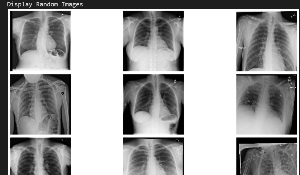
Data visualization
Using the image names listed in the csv file, you can retrieve the image associated with each row of data in the data frame. Run the following cells to visualize randomly selected images from the dataset.
# Extract numpy values from Image column in data frame
images = train_df['Image'].values

# Extract 9 random images from it
random_images = [np.random.choice(images) for i in range(9)]
# #numpy.random.choice(a, size=None, replace=True, p=None)
#Randomly extract numbers from a (as long as it is ndarray, but it must be one-dimensional) and form an array of specified size
#replace:True means the same number can be taken, False means the same number cannot be taken
#Array p: corresponding to array a, indicating the probability of taking each element in array A. by default, the probability of selecting each element is the same.

# Location of the image dir
img_dir = 'nih/images-small/'

print('Display Random Images')

# Adjust the size of your images
plt.figure(figsize=(20,10))

# Iterate and plot random images
for i in range(9):
    plt.subplot(3, 3, i + 1)
    img = plt.imread(os.path.join(img_dir, random_images[i]))
    # Key plt can also directly read the image and return numpy array see  https://matplotlib.org/api/_as_gen/matplotlib.pyplot.imread.html
    plt.imshow(img, cmap='gray')
    plt.axis('off')

# Adjust subplot parameters to give specified padding
plt.tight_layout()
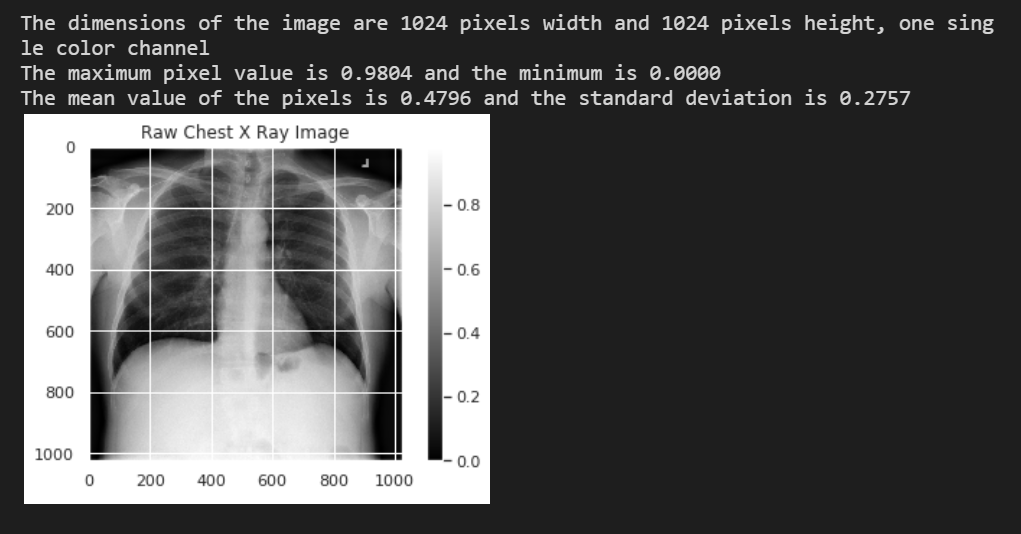
Investigate a single image
Run the following cells to view the first image in the dataset and print out some details of the image content.
# Get the first image that was listed in the train_df dataframe
sample_img = train_df.Image[0]
raw_image = plt.imread(os.path.join(img_dir, sample_img))
plt.imshow(raw_image, cmap='gray')
plt.colorbar()
plt.title('Raw Chest X Ray Image')
print(f"The dimensions of the image are {raw_image.shape[0]} pixels width and {raw_image.shape[1]} pixels height, one single color channel")
print(f"The maximum pixel value is {raw_image.max():.4f} and the minimum is {raw_image.min():.4f}")
print(f"The mean value of the pixels is {raw_image.mean():.4f} and the standard deviation is {raw_image.std():.4f}")
- List item
Survey pixel value distribution
Run the following cells to plot the distribution of pixel values in the above figure.
Add the usage of seaborn https://blog.csdn.net/qq_34264472/article/details/53814653
# Plot a histogram of the distribution of the pixels
sns.distplot(raw_image.ravel(),
             label=f'Pixel Mean {np.mean(raw_image):.4f} & Standard Deviation {np.std(raw_image):.4f}', kde=False)
plt.legend(loc='upper center')
plt.title('Distribution of Pixel Intensities in the Image')
plt.xlabel('Pixel Intensity')
plt.ylabel('# Pixels in Image')

Image preprocessing in Keras
Before training, you will first modify the image to make it more suitable for training convolutional neural network. For this task, you will use the Keras ImageDataGenerator function to perform data preprocessing and data enhancement.
Run the next two cells to import this function and create an image generator for preprocessing.
# Import data generator from keras
from keras.preprocessing.image import ImageDataGenerator
# Normalize images
image_generator = ImageDataGenerator(
    samplewise_center=True, #Set each sample mean to 0.
    samplewise_std_normalization= True # Divide each input by its standard deviation
)
Variance: image created above_ The generator will adjust your image data so that the new average value of the data is 0 and the standard deviation of the data is 1. In other words, the generator replaces each pixel value in the image
The new value calculated by subtracting the mean and dividing by the standard deviation
Run next cell to use image_ The generator preprocesses your data.
In this step, you will also reduce the image size to 320x320 pixels.
# Flow from directory with specified batch size and target image size
generator = image_generator.flow_from_dataframe(
        dataframe=train_df,
        directory="nih/images-small/",
        x_col="Image", # features
        y_col= ['Mass'], # labels
        class_mode="raw", # 'Mass' column should be in train_df
        batch_size= 1, # images per batch
        shuffle=False, # shuffle the rows or not
        target_size=(320,320) # width and height of output image
)
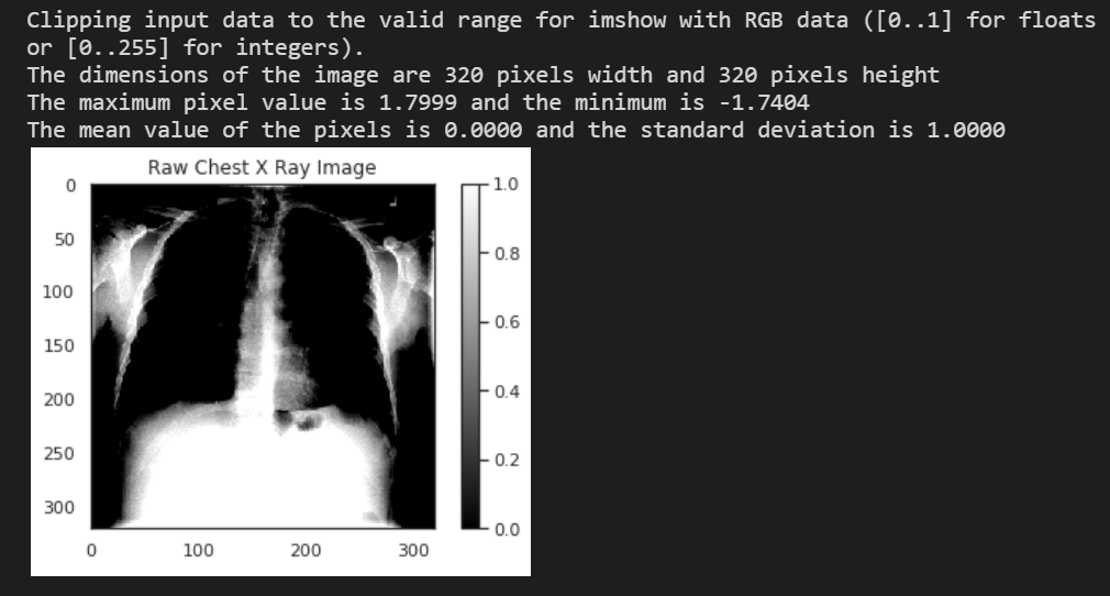
Example of running the next cell to draw a preprocessed image:
# Plot a processed image
sns.set_style("white")
generated_image, label = generator.__getitem__(0)
plt.imshow(generated_image[0], cmap='gray')
plt.colorbar()
plt.title('Raw Chest X Ray Image')
print(f"The dimensions of the image are {generated_image.shape[1]} pixels width and {generated_image.shape[2]} pixels height")
print(f"The maximum pixel value is {generated_image.max():.4f} and the minimum is {generated_image.min():.4f}")
print(f"The mean value of the pixels is {generated_image.mean():.4f} and the standard deviation is {generated_image.std():.4f}")
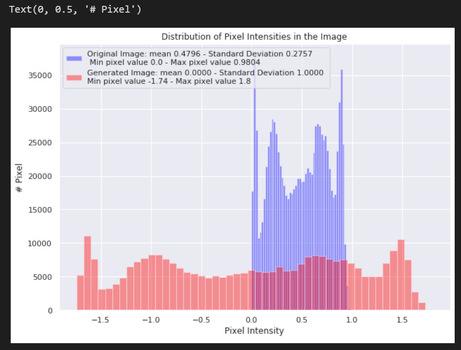
Run the following cells to see a comparison of the pixel value distribution in the new preprocessed image with the original image.
# Include a histogram of the distribution of the pixels
sns.set()
plt.figure(figsize=(10, 7))

# Plot histogram for original iamge
sns.distplot(raw_image.ravel(),
             label=f'Original Image: mean {np.mean(raw_image):.4f} - Standard Deviation {np.std(raw_image):.4f} \n '
             f'Min pixel value {np.min(raw_image):.4} - Max pixel value {np.max(raw_image):.4}',
             color='blue',
             kde=False)

# Plot histogram for generated image
sns.distplot(generated_image[0].ravel(),
             label=f'Generated Image: mean {np.mean(generated_image[0]):.4f} - Standard Deviation {np.std(generated_image[0]):.4f} \n'
             f'Min pixel value {np.min(generated_image[0]):.4} - Max pixel value {np.max(generated_image[0]):.4}',
             color='red',
             kde=False)

# Place legends
plt.legend()
plt.title('Distribution of Pixel Intensities in the Image')
plt.xlabel('Pixel Intensity')
plt.ylabel('# Pixel')