1. regression
1.1 origin and definition
Regression was first proposed by Galton. Through his research, he found that: if the parents are taller, the height of the children will be lower than the average height of the parents; On the contrary, if both parents are shorter, the height of their children is higher than the average height of their parents. He believes that there is a binding force in nature, so that the distribution of height will not develop to the two extremes of height, but tend to return to the center, so it is called regression.
At present, it is defined as a numerical (scalar) prediction technology from the perspective of usage, which is different from classification (category prediction technology).
1.2 different usage
1.2.1 Explanation
Regression can be used for empirical research to study the internal relationship and law between independent variables and dependent variables, which is common in social science research.
- Does the popularity of the Internet reduce educational inequality?
- What are the influencing factors of College Students' employment choice?
- What are the influencing factors of customer satisfaction in the medical e-commerce scenario?
1.2.2 Prediction
Regression can also be used to make predictions and accurately predict unknown things based on known information.
- Stock market forecast: forecast the average value of the stock market tomorrow according to the changes of stocks in the past 10 years, news consulting, corporate M & a consulting, etc.
- Product recommendation: predict the possibility of a user purchasing a product according to the user's past purchase records and candidate product information.
- Automatic driving: predict the correct steering wheel angle according to the data of various sensor s of the vehicle, such as road conditions and vehicle distance.
1.3 model construction
Whether the purpose is interpretation or prediction, we need to master the laws related to the task (understanding the world), that is, to establish a reasonable model.
The difference is that the interpretation model only needs to be constructed based on the training set, and generally has an analytical solution (Econometric Model). The prediction model must be tested and adjusted on the test set. Generally, it does not have analytical solution, and the parameters need to be adjusted by machine learning. Therefore, with the same model framework and data set, the optimal interpretation model and prediction model are likely to be different.
This paper mainly focuses on the construction of prediction model, and does not further involve the content related to interpretation model.
2. Model construction based on machine learning
We take the task of Combat Power of a pokemon as an example to sort out the details of the three steps of machine learning.
- Input: CP value before evolution, species (Bulbasaur), blood volume (HP), Weight (Weight), Height (Height)
- Output: CP value after evolution

2.1 model assumptions - linear model
For convenience, we choose the simplest linear model as the model framework to complete the regression task. We can use single feature or multi feature linear regression models, which will be more complex and the model set will be larger.

In order to select a reasonable model framework, it is necessary to explore the data set in advance and observe the relationship between variables, which will determine which variables are finally put into the model and whether the variables need to be processed again (quadratic term, reciprocal, etc.).
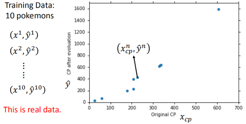
It can be seen that the horizontal axis and vertical axis are mainly linear, and there are also some quadratic relations (quadratic terms can be considered).
Model framework (preset) + parameters (to be estimated) = model (target)
At present, the parameters of the model include the weight of each feature \ (w_i \) and the offset \ (b \).
2.2 model evaluation - loss function
The regression task described in this paper belongs to a supervised learning scenario, so it is necessary to collect enough input and output pairs to guide the construction of the model.

With these real data, how can we measure the quality of the model? From a mathematical point of view, we use the Loss function to measure the quality of the model. The Loss function is set based on the difference between the predicted value and the actual value of the model.

In this paper, we choose the commonly used mean square error as the loss function.
2.3 model tuning - gradient descent
When the model is non convex, there is no analytical solution, so it can only be optimized iteratively by heuristic method. The commonly used method is gradient descent.

First, we randomly select a \ (w^0 \), then calculate the differential to determine the moving direction, and then update the corresponding parameters and cycle until the lowest point is found (the difference between the two updates is less than the threshold or reaches the preset number of iterations).
For the model with multiple parameters to be updated, the steps are basically the same, except for partial differentiation.

In the process of gradient descent, some problems will be encountered, resulting in the inability to achieve the best.

How to solve these problems will be involved in the future.
3. Problems and solutions in model construction
3.1 Generalization of evaluation model
A good model should perform well not only in the training set, but also in the unknown data set (test set, real application scenario).
Therefore, we must calculate the performance of the model on the tester. Ideally, there can be no large decline.

3.2 improve the fitting degree of the model
If the model is too simple, the model set is small and may not contain the real model, that is, there is an under fitting problem.
We can choose more complex models to optimize performance. As an example, the prediction performance is significantly improved.

We can also add adjustment items (Pokemon types) to the model to improve the model.

The performance of the model in the training set and test set is as follows:

3.3 prevent overfitting
If we continue to use higher-order models, fitting problems may occur.

We can prevent the over fitting problem by adding regular terms.

The influence of regular term weight change on model performance is as follows:

4. Regression - code demonstration
Now suppose there are 10 x's_ Data and y_data, the relationship between X and Y is y_data=b+w*x_data. b. W are parameters that need to be learned. Now let's practice finding B and W with gradient descent.
import numpy as np
import matplotlib.pyplot as plt
from pylab import mpl

# matplotlib has no Chinese font, which can be solved dynamically
plt.rcParams['font.sans-serif'] = ['Simhei']  # Display Chinese
mpl.rcParams['axes.unicode_minus'] = False  # Solve the problem that the negative sign '-' is displayed as a square in the saved image

# Generate experimental data
x_data = [338., 333., 328., 207., 226., 25., 179., 60., 208., 606.]
y_data = [640., 633., 619., 393., 428., 27., 193., 66., 226., 1591.]
x_d = np.asarray(x_data)
y_d = np.asarray(y_data)
x = np.arange(-200, -100, 1) # The candidate of the parameter refers to the offset item b
y = np.arange(-5, 5, 0.1) # The candidate of the parameter refers to the weight w
Z = np.zeros((len(x), len(y)))
X, Y = np.meshgrid(x, y)

# The loss under each possible combination needs to be calculated 100 * 100 = 10000 times
for i in range(len(x)):
    for j in range(len(y)):
        b = x[i]
        w = y[j]
        Z[j][i] = 0  # meshgrid spits out the result: y is the row and x is the column
        for n in range(len(x_data)):
            Z[j][i] += (y_data[n] - b - w * x_data[n]) ** 2
        Z[j][i] /= len(x_data)
The above code generates the experimental data, and uses the exhaustive method to calculate the loss of all possible combinations, of which the minimum value is 10216.
Next, we try to use the gradient descent method to quickly find the smaller loss value.
# linear regression
b=-120
w=-4
lr = 0.000005
iteration = 10000 #Set to 10000 first

b_history = [b]
w_history = [w]
loss_history = []
import time
start = time.time()
for i in range(iteration):
    m = float(len(x_d))
    y_hat = w * x_d  +b
    loss = np.dot(y_d - y_hat, y_d - y_hat) / m
    grad_b = -2.0 * np.sum(y_d - y_hat) / m
    grad_w = -2.0 * np.dot(y_d - y_hat, x_d) / m
    # update param
    b -= lr * grad_b
    w -= lr * grad_w

    b_history.append(b)
    w_history.append(w)
    loss_history.append(loss)
    if i % 1000 == 0:
        print("Step %i, w: %0.4f, b: %.4f, Loss: %.4f" % (i, w, b, loss))
end = time.time()
print("About time required:",end-start)
# Step 0, w: 1.6534, b: -119.9839, Loss: 3670819.0000
# Step 1000, w: 2.4733, b: -120.1721, Loss: 11492.1941
# Step 9000, w: 2.4776, b: -121.6771, Loss: 11435.5676
It can be found that the gradient descent method can quickly iterate from the initial value to the appropriate parameter combination, which is close to the optimal parameter. However, we find that the process of reaching the optimal value is very slow. The following code can be used to visualize the optimization process.
# plot the figure
plt.contourf(x, y, Z, 50, alpha=0.5, cmap=plt.get_cmap('jet'))  # Fill contour
plt.plot([-188.4], [2.67], 'x', ms=12, mew=3, color="orange") # Optimal parameters
plt.plot(b_history, w_history, 'o-', ms=3, lw=1.5, color='black')
plt.xlim(-200, -100)
plt.ylim(-5, 5)
plt.xlabel(r'$b$')
plt.ylabel(r'$w$')
plt.title("linear regression")
plt.show()
As shown in the figure below, the final optimization direction of parameters is correct, but it is stopped in advance because the number of iterations is not enough.

We changed the number of iterations to 100000, and the results are as follows:

The number of iterations is still insufficient. We continue to change the number of iterations to 1 million, and the result is close to the optimal, as shown below:

Too many iterations will consume too many computing resources. We can speed up the speed by adjusting the learning rate. When we set the learning rate to twice the previous (0.00001), 100000 iterations can achieve near optimal results, as shown below;

However, it should be noted that if the learning rate is set too high, it may oscillate and cannot converge. The following figure shows the situation when we set the learning rate to 0.00005.

In a word, we should understand the powerful ability and instability of machine learning, and then learn the relevant principles and use them skillfully.