Introduction to MNE Python series, continuously updated

0. What is MNE?

Frankly speaking, MNE is the strongest physiological signal analysis artifact I have ever used (maybe I have little knowledge, don't spray it), and the processing range covers EEG, MEG and other types.

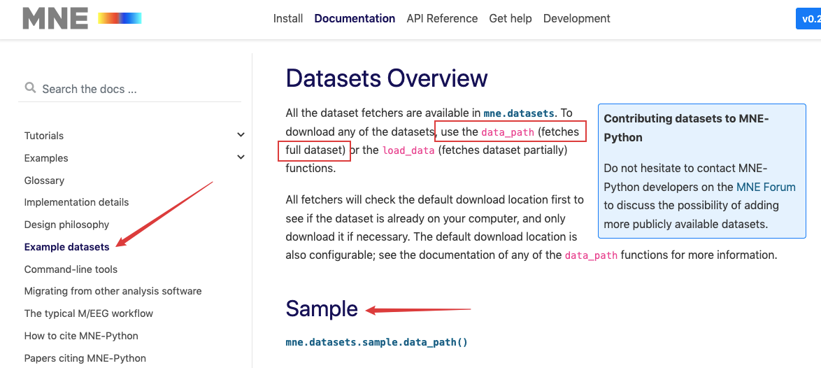
MNE is essentially an open source Python third-party library / module, I think MNE official website The introduction on the front page is the most accurate overview of MNE, as shown in the figure:

1. Article ideas

Because MNE has many functions, including reading data sets, preprocessing, classification, visualization and other complete processes, I can't introduce them all. Based on the principle that giving fish is better than giving fish, I decided that the idea of the first article in this series is to introduce a simple sample demo in detail and show the general process of using MNE.

2. MNE installation

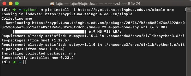
Like all other Python third-party libraries / modules, you can use pip install mne to install them. I won't repeat it too much (here I use the Tsinghua image source):

3. MNE code practice

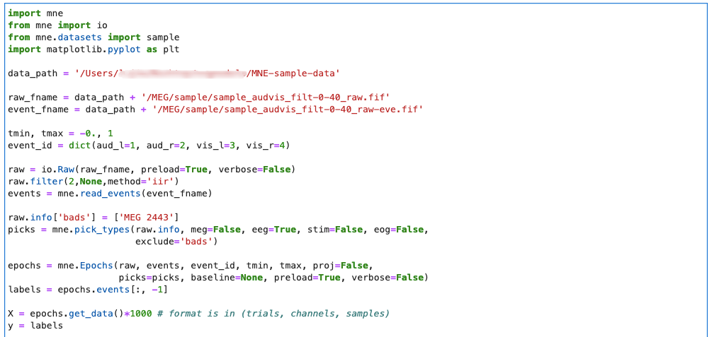
First post a MNE code. If you don't know MNE before, you should be confused at the moment. It's not a big problem. Next, I'll take you to analyze all the codes line by line. Let's Go!:

Import MNE related packages

import mne
from mne import io
from mne.datasets import sample

# Data visualization package
import matplotlib.pyplot as plt

Import dataset

There are two ways to import a dataset:

1) Remote download dataset

In the previous step, we have used from MNE Datasets import sample imports the sample dataset. Note: here sample is the name of a dataset! (the introduction of this data set is at the end of the text)

Then we can use data_path() gets all the data in this data set:

data_path = sample.data_path()

2) Locally downloaded dataset

# Custom data set storage location
data_path = '/Users/xxx/xxx/MNE-sample-data'

Create data object

One of the data structures of MNE is the raw data structure, which creates raw data objects in the following ways:

# Set relevant parameters
raw_fname = data_path + '/MEG/sample/sample_audvis_filt-0-40_raw.fif' 
event_fname = data_path + '/MEG/sample/sample_audvis_filt-0-40_raw-eve.fif'
tmin, tmax = -0., 1
event_id = dict(aud_l=1, aud_r=2, vis_l=3, vis_r=4)

# Use 1): preload=False, use 2): preload=True
raw = io.Raw(raw_fname, preload=True, verbose=False)

Through print , we can find that the core data is n_channels and times:

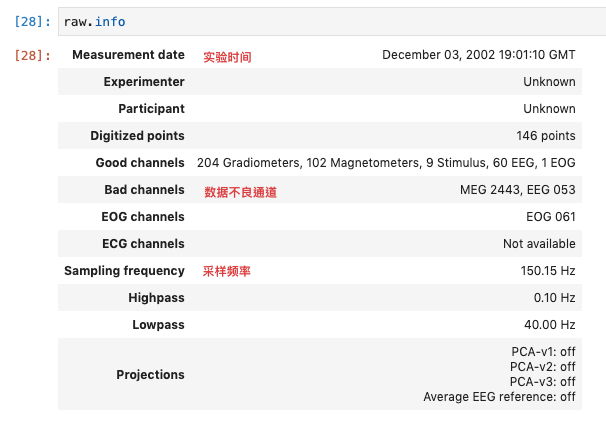
You can also use raw Info to view the specific information of raw data:

raw.filter(2, None, method='iir')  # Filtering using iir filter
events = mne.read_events(event_fname)

raw.info['bads'] = ['MEG 2443']    # Set bad channel

# Select channels by type and name
picks = mne.pick_types(raw.info, meg=False, eeg=True, stim=False, eog=False,
                       exclude='bads') 

Create epochs

Splitting data into Epochs can facilitate neural network processing. There is an Epochs class in MNE. We can directly extract Epochs from raw data objects through this class of methods:

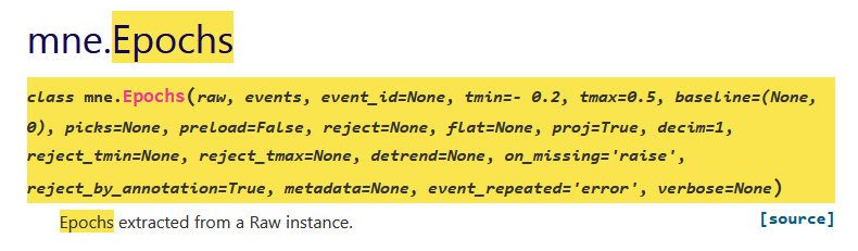
# Create an object of epochs class and pass in the previously set parameters, (tmin,tmax) as the time length of each trial in epochs
epochs = mne.Epochs(raw, events, event_id, tmin, tmax, proj=False,
                    picks=picks, baseline=None, preload=True, verbose=False)
labels = epochs.events[:, -1]

Extract data

X = epochs.get_data()*1000 
Y = labels

get_ The format of data returned by data() is (trials, channels, samples), and the output through print(X.shape) is (278,61150):
It corresponds to 277.7s (data duration) / 1s (time length of each trial), number of channels (60EEG+1EOG) and sampling frequency (150Hz).

Data visualization

MNE integrates many ready-made functions, which can realize many complex functions with a simple line of code. Let's take some pictures to experience:

# Analyze data within 0-1s
import matplotlib.pyplot as plt

raw.info['bads'] = ['MEG 2443']  
picks = mne.pick_types(raw.info, meg=False, eeg=True, stim=False, eog=False,
                       exclude='bads')
t_idx = raw.time_as_index([-0., 1.])
data, times = raw[picks, t_idx[0]:t_idx[1]]

plt.plot(times,data.T)

# Plot the power spectral density of each channel
raw.plot_psd()
plt.show()

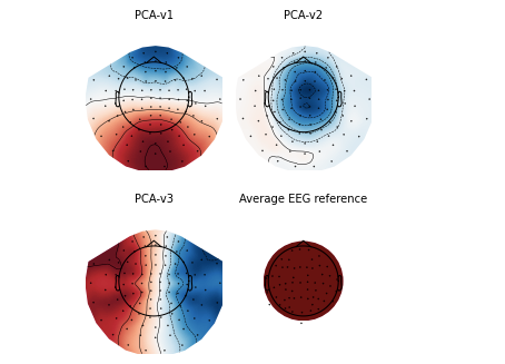
# Draw SSP vector diagram
raw.plot_projs_topomap()
plt.show()

4. Introduction to sample dataset

data acquisition

The data set was obtained by the Neuromag Vectorview system at the Athinoula A. Martino biomedical imaging center at MGH/HMS/MIT (Massachusetts General Hospital). MEG (magnetoencephalogram) data of 60 channel electrode caps were collected at the same time. The original MRI (nuclear magnetic resonance) data set was obtained by using Siemens 1.5 T Sonata scanner with MPRAGE sequence.

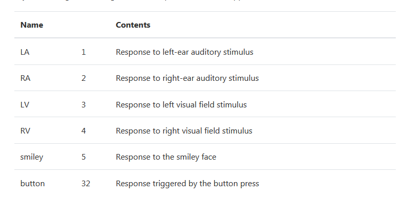
Experimental setup

In the experiment, checkerboard patterns appeared in the subjects' left and right visual fields, accompanied by tones in the left and right ears, with a stimulation interval of 750 ms. In addition, the smiling face pattern will appear randomly in the center of the subject's visual field. The subject is required to press the button with the right index finger as soon as possible after the smiling face appears. The corresponding relationship between stimulus and response in the experiment is as follows:

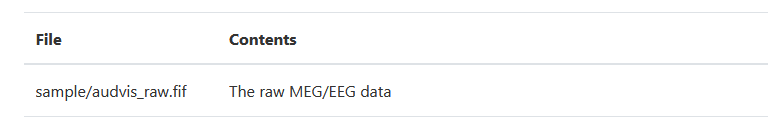
Dataset content

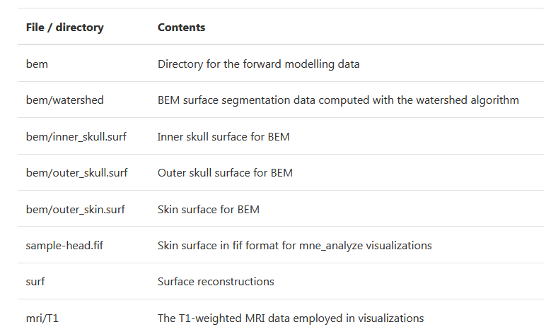
The Sample data set mainly includes two parts: MEG/sample (MEG/EEG data) and MRI reconstruction data subjects/sample from another subject. We mainly use the former, and its directory is as follows:

Conclusion

Ok, a small demo of MNE has been interpreted here. Maybe you have felt the power and simplicity of MNE. I will sort out various classes and functions in MNE in subsequent articles. If you are interested, please pay attention and go again ^ ^ ^!!