Hello, I'm a graduate student from the ECG group of Hebei University. This article is my understanding and sharing of mnist recognition learning.

This paper is mainly used to give a guide to students who want to build a network with keras to identify mnist.

Please correct any mistakes

I will accept it with an open mind

The first is the installation of the library. The version I selected is tensorflow GPU version 2.6.0. If you are the same as my version, you can directly copy the above code to import the library.

from tensorflow.keras.datasets import mnist
from tensorflow.keras import models,layers
from tensorflow.keras.utils import to_categorical
from tensorflow.keras import optimizers
import numpy as np
import matplotlib.pyplot as plt
from PIL import Image

First, let's look at the first step: dataset import and processing

#Download MNIST dataset
(train_datas,train_labels),(test_datas,test_labels)=mnist.load_data()

#The data sets were preprocessed and normalized
train_datas=train_datas.reshape((60000,28,28,1))
train_datas=train_datas.astype('float32')/255
test_datas=test_datas.reshape((10000,28,28,1))
test_datas=test_datas.astype('float32')/255

#Heat code labels
train_labels=to_categorical(train_labels)
test_labels=to_categorical(test_labels)

We first download the data through the MNIST data set in the keras library. The data has helped us divide the training set and the test set. The training set has 60000 pictures and the test set has 10000 pictures, all of which are 28 × 28 pixel single channel grayscale image.

Then we need to normalize the images of the training set and the test set. Why should we normalize them?

The value of the picture is between 0 and 255. The reason why we divide the picture by 255 is to make all the values of the picture become 0 ~ 1, so that the classifier can better classify in our subsequent network.

The next step is to heat code the labels of the data set. This step is basically necessary to make the calculation of the distance between features more reasonable. Students who can't understand can directly remember this step

Step 2: partition of verification set

#K-fold cross validation
k=4
num_val_samples=len(train_datas)//k
for i in range(k):
    print('processing fold #',i)
    val_train_datas=train_datas[i*num_val_samples:(i+1)*num_val_samples]
    val_train_labels=train_labels[i*num_val_samples:(i+1)*num_val_samples]

    partial_train_datas=np.concatenate(
        [train_datas[:i*num_val_samples],
         train_datas[(i+1)*num_val_samples:]],
        axis=0
    )
    partial_train_labels=np.concatenate(
        [train_labels[:i*num_val_samples],
         train_labels[(i+1)*num_val_samples:]],
        axis=0
    )

Here we use K-fold cross validation to divide the training set into validation sets. You can refer to other materials for learning the principle of K-fold cross validation

Step 3: build a network model

#Define network model
def network():
    model=models.Sequential()
    model.add(layers.Conv2D(16,(3,3),activation='relu',input_shape=(28,28,1)))
    model.add(layers.Conv2D(32,(3,3),activation='relu',padding='same'))
    model.add(layers.MaxPooling2D(2,2))
    model.add(layers.Dropout(0.5))
    model.add(layers.Conv2D(32,(3,3),activation='relu',padding='same'))
    model.add(layers.Conv2D(64,(3,3),activation='relu',padding='same'))
    model.add(layers.MaxPooling2D(2,2))
    model.add(layers.Dropout(0.5))
    model.add(layers.Conv2D(64,(3,3),activation='relu',padding='same'))
    model.add(layers.MaxPooling2D(2,2))
    model.add(layers.Dropout(0.5))
    model.add(layers.Flatten())
    model.add(layers.Dense(512,activation='relu'))
    model.add(layers.Dense(10,activation='softmax'))
    model.compile(optimizer=optimizers.RMSprop(learning_rate=0.001),
                  loss='categorical_crossentropy',
                  metrics=['accuracy'])
    return model

This model is gradually improved by me based on the CNN convolutional neural network model. Don't think it is difficult to build the network. We generally build the network from a very small network, and then constantly adjust the network super parameters and add other layers to optimize the network performance.

First of all, the first step to build a model with keras is to add Sequential (). The purpose of this step is to define a network framework so that we can have a container to put other layers in it.

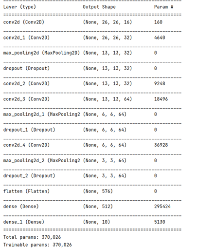
Next, we add the convolution layer and pooling layer to this framework. If you don't know the parameters of Conv2D convolution layer, you can solve them by referring to other materials. In the first layer of the network, we need to set the input shape, because the picture of our MNIST dataset is 28 × 28 pixel single channel picture, so here is input_shape we set to (28,28,1)

To activate the function, we select the ReLU function

In order to prevent over fitting of the model and improve the classification performance of the network model, we add a Dropout layer to the network to round off some parameters. Here, Dropout is set to 0.5 to round off 50%.

After flattening the tile layer, it is sent to the Dense layer for feature extraction, and the extracted features are sent to the softmax classifier for classification. The reason why the parameter is set to 10 in the last layer of Dense is that there are 10 different categories from 0 to 9 in MNIST, so we set it to 10 here. If there are 5 categories, it is set to 5, and the second classification is set to 2. However, the classifiers of the second classification are mostly classified by Sigmoid.

After the network is built, we want the network to adjust the super parameters to correct the deviation. How to do it?

This requires setting the optimizer and loss function in the network. The working principle can be queried by beeping or other websites.

The optimizer selects REMprop, and the learning rate is set to 0.001, which can also be expressed as 1e-3,

Loss function selection category_ Cross entropy loss function

Now let's print the network model. You don't need to print this when you write it yourself

  Step 4: start training

#Construct network for training
model=network()
history=model.fit(partial_train_datas,partial_train_labels,epochs=60
                  ,batch_size=512,
                  validation_data=(val_train_datas,val_train_labels))

Well, let's start training the network now. Because our network is built with a function definition, we must first call this function and then start training.  

The data we use for training is the training set after the verification set is divided. We can adjust the number of iterations at will. Here, we set the number of iterations to 60, which is the best number of iterations determined after many adjustments, which is between the critical point of over fitting and under fitting.

We set 512 batches as a batch, which means that 512 batches are sent to the network for training each time. The verification set of the network is the verification set divided by our previous K-fold cross verification.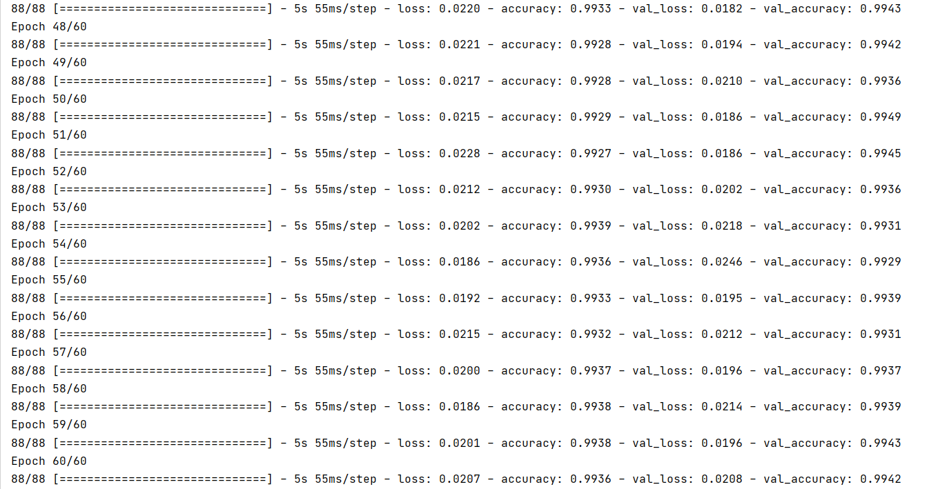

 

Step 5: draw an image

#Draw loss image
history_dict=history.history
loss_values=history_dict['loss']
val_loss_values=history_dict['val_loss']
epochs=range(1,len(loss_values)+1)
plt.plot(epochs,loss_values,'bo',label='train loss')
plt.plot(epochs,val_loss_values,'b',label='Validation loss')
plt.title('Training and Validation loss')
plt.xlabel('Epochs')
plt.ylabel('Loss')
plt.legend()

#Rendering accuracy image
plt.figure()
history_dict=history.history
acc_values=history_dict['accuracy']
val_acc_values=history_dict['val_accuracy']
epochs=range(1,len(loss_values)+1)
plt.plot(epochs,acc_values,'ro',label='train acc')
plt.plot(epochs,val_acc_values,'r',label='Validation acc')
plt.title('Training and Validation acc')
plt.xlabel('Epochs')
plt.ylabel('acc')
plt.legend()
plt.show()

Here, we can choose to draw the change curves of Loss and Accuracy to facilitate us to observe the performance changes of our network more intuitively. You can choose to draw or not. What does each parameter mean? We need to consult and learn by ourselves.

 

 

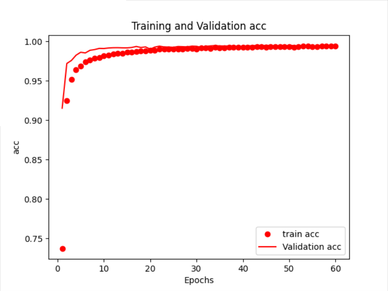
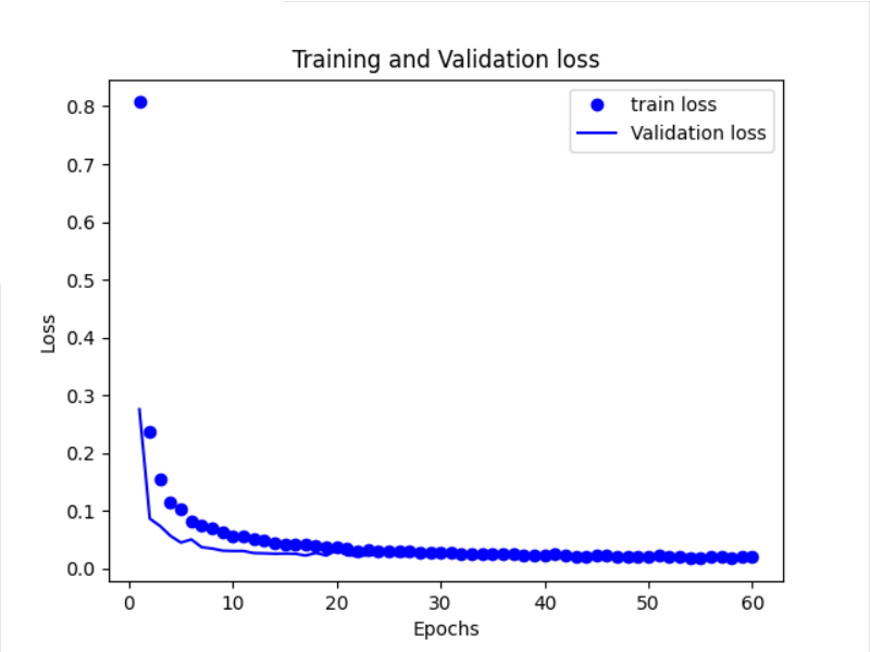
Through the image, we can see that the Loss and Accuracy on the training set and the verification set basically coincide, which proves that the critical point of our model is found well.

We input the test set into the network for the final test to see the results

#Verify performance on test set
test_loss,test_acc=model.evaluate(test_datas,test_labels)
print('test_acc:{}',format(test_acc))
print('test_loss:{}'.format((test_loss)))

The accuracy on the test set is very high, which shows that our network is built successfully. We need to constantly increase or decrease the number of network layers and adjust the super parameters to find the optimal model, which needs to be done slowly.

After training the network, let's input a handwritten picture to see how the recognition effect is

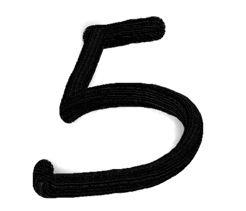
  This is a picture written by myself with drawing software on the computer. Note that the color of our picture is just opposite to that of MNIST. The pictures in MNIST are white words on a black background. We usually have black words on a white background, so we need a piece of code to adjust the color later. Emphasize that 0 represents white and 255 represents black in the image

#import picture
img_path=r'D:\python interpreter\pycharm environment\pythonProject3\data\MNIST\com-5.png'
image=Image.open(img_path)
#Change picture to 28 × 28 pixels
image=image.resize((28,28),Image.ANTIALIAS)
#Convert picture to single channel grayscale
image=image.convert('L')
#Convert grayscale image to numpy array
image_rr=np.array(image.convert('L'))
#Loop traversal, turning white into black and black into white in the picture
for i in range(28):
    for j in range(28):
        if image_rr[i][j]<100:
            image_rr[i][j]=255
        else:
            image_rr[i][j]=0
#The image is normalized again
image_rr=image_rr/255
#Convert the image to a form suitable for network input
image_rr=np.reshape(image_rr,(1,28,28,1))
#Put the picture into the network for prediction
result=model.predict(image_rr)
#Arrange the results horizontally and take the maximum value
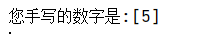
pred=np.argmax(result,axis=1)

print('Your handwritten number is:{}'.format(pred))

OK, let's take a look at the recognition effect

  Here, the whole content of this article is over. You are welcome to correct any mistakes.

In addition, the network in this paper can only recognize the numbers written on the computer or mobile phone drawing board, and the photos written on paper will not be recognized in the network. The preliminary analysis shows that there is no handwriting written on paper in MNIST data set, so some features of the network can not be extracted, resulting in recognition errors.

Thank you for your click support.