introduction

Based on PyTorch framework, this paper uses CNN convolutional neural network to realize MNIST handwritten numeral recognition, which runs only on CPU.

Four structures, Linear pure Linear layer, CNN convolutional neural network, Inception network and Residual residual network, have been used to recognize handwritten digits from MNIST data sets, and their recognition accuracy has been compared and analyzed. (the other three have not been released yet)

After watching the video of the boss of station B, and just a course experiment of in-depth learning is handwritten numeral recognition, record this blog.
This article is written by the author word by word. I believe it has been very detailed and can be used for beginners. You are welcome to put forward your opinions and improvements!

Import package:

import torch
import numpy as np
from matplotlib import pyplot as plt
from torch.utils.data import DataLoader
from torchvision import transforms
from torchvision import datasets
import torch.nn.functional as F

1, Dataset (MNIST)

MNIST data set is a very classic data set in the field of machine learning. It is composed of 60000 training samples and 10000 test samples. Each sample is a 28 * 28 pixel gray handwritten numeral picture.

Download:
Official website: http://yann.lecun.com/exdb/mnist/
Network disk address: MNIST dataset (extraction code: zm7q)

There are 4 files in total, including training set, training set label, test set and test set label

File name	size	content
train-labels-idx1-ubyte.gz	9,681 kb	55000 training sets and 5000 verification sets
train-labels-idx1-ubyte.gz	29 kb	Tags corresponding to training set pictures
t10k-images-idx3-ubyte.gz	1,611 kb	10000 test sets
t10k-labels-idx1-ubyte.gz	5 kb	Label corresponding to the test set picture

1.1 reading MNIST dataset

The data downloaded directly cannot be opened through decompression or application program, because these files are not in any standard image format, but stored in bytes, so you must write a program to open it.

torchvision. The datasets package already contains MNIST datasets, which can be obtained by entering code in the compiler. The steps are as follows:

• Step 1: normalization, softmax normalization exponential function( https://blog.csdn.net/lz_peter/article/details/84574716 ), where 0.1307 is the mean and 0.3081 is the std standard deviation

transform = transforms.Compose([transforms.ToTensor(), transforms.Normalize((0.1307,), (0.3081,))])

• Step 2: Download / obtain the data set, where root is the storage path of the data set, train=True is the training set, otherwise it is the test set.

train_dataset = datasets.MNIST(root='./data/mnist', train=True, download=True, transform=transform)  
test_dataset = datasets.MNIST(root='./data/mnist', train=False, download=True, transform=transform)  # train=True training set, = False test set

• Step 3: after instantiating a dataset, package it with Dataloader, that is, load the dataset. Batch here_ Size is a super parameter, see section 5 for details; shuffle=True means to disrupt the data set. Here, we disrupt the training set for training and test the test set sequentially.

train_loader = DataLoader(train_dataset, batch_size=batch_size, shuffle=True)
test_loader = DataLoader(test_dataset, batch_size=batch_size, shuffle=False)

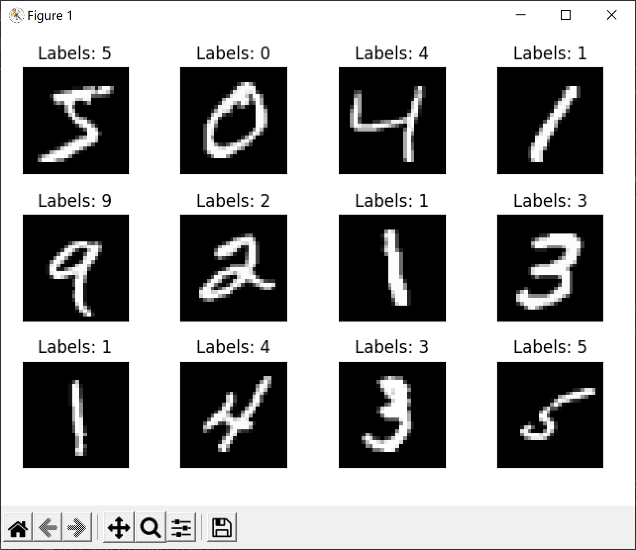
1.2 display MNIST dataset:

Here are 12 pictures, including picture content and labels.

fig = plt.figure()
for i in range(12):
    plt.subplot(3, 4, i+1)
    plt.tight_layout()
    plt.imshow(train_dataset.train_data[i], cmap='gray', interpolation='none')
    plt.title("Labels: {}".format(train_dataset.train_labels[i]))
    plt.xticks([])
    plt.yticks([])
plt.show()

Output results:

2, Building models (CNN)

2.1 convolution

The number of channels of each convolution kernel shall be the same as the number of input channels, and the total number of convolution kernels shall be the same as the number of output channels.
After convolution, C(Channels) changes, W(width) and H(Height) are variable and invariable, depending on the padding.

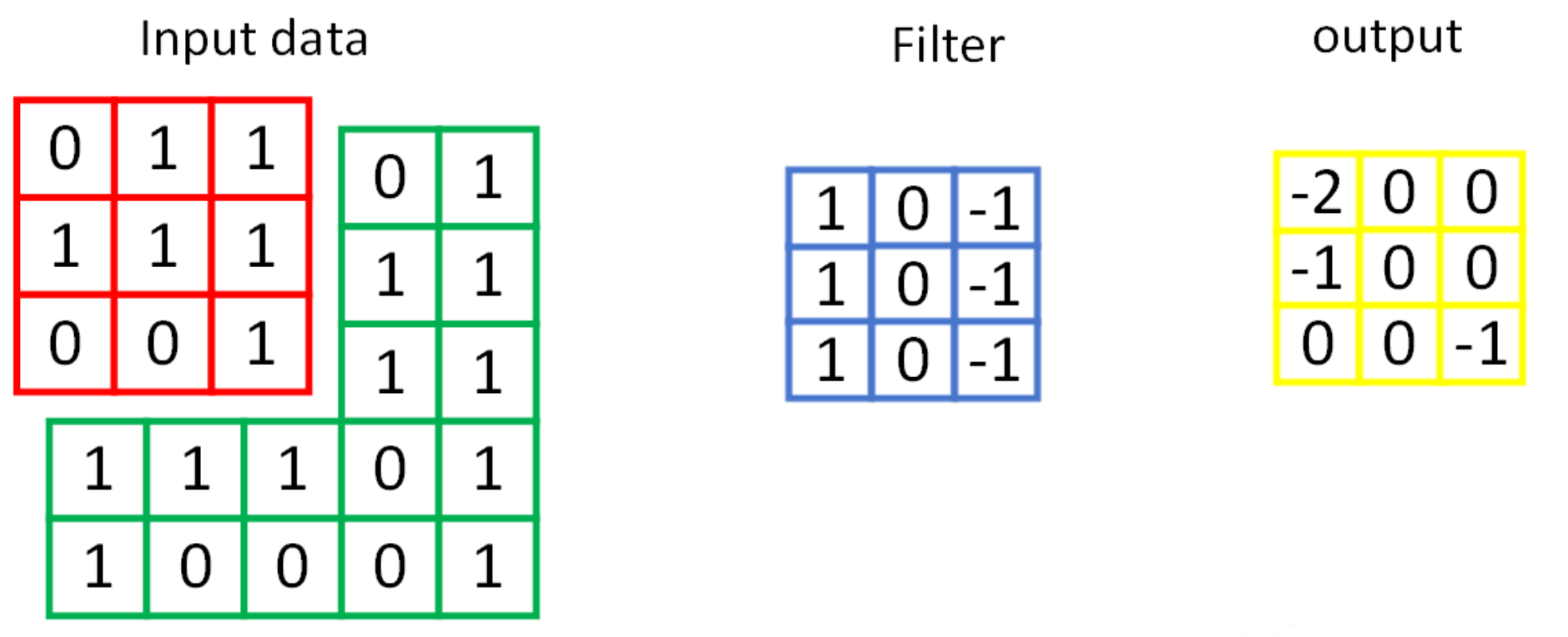
torch.nn.Conv2d(in_channels, out_channels, kernel_size, stride, padding)

Parameters:

• in_channels: input channels
• out_channels: output channels
• kernel_size: convolution kernel size
• Stripe: step size
• padding: filling

2.2 activation layer

The activation layer uses the ReLU activation function.
Linear rectified unit (relu), also known as modified linear unit, is an activation function commonly used in artificial neural networks. It usually refers to the nonlinear function represented by slope function and its variants.

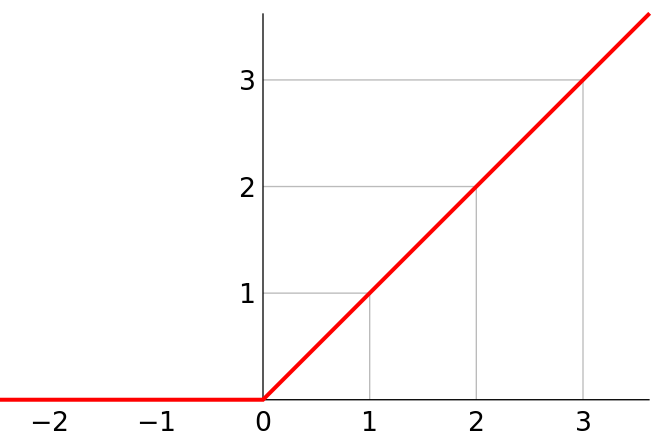
torch.nn.ReLU()

2.3 pool layer

The pooling layer adopts maximum pooling.
After pooling, C(C.hannels) remained unchanged, W(width) and H(Height) changed.

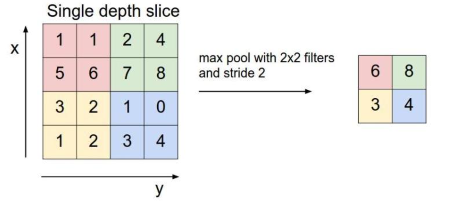
torch.nn.MaxPool2d(input, kernel_size, stride, padding)

Parameters:

• Input: input
• kernel_size: convolution kernel size
• Stripe: step size
• padding: filling

2.4 full connection layer

Before, the convolution layer requires that the input and output are four-dimensional tensors (B,C,W,H), while the input and output of the full connection layer are two-dimensional tensors (B,Input_feature). After convolution, activation and pooling, use view to flatten and enter the full connection layer.

2.5 CNN model

The model is shown in the figure:

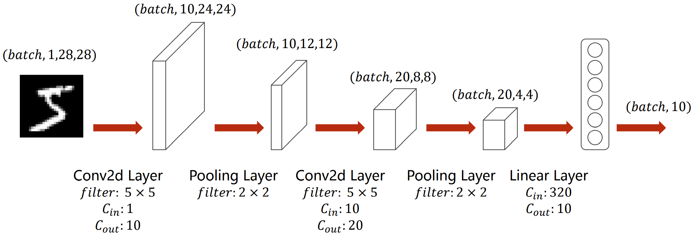
For example, if you input an image with handwritten numeral "5", its dimension is (batch,1,28,28), that is, the height and width of a single channel are 28 pixels respectively.

• Firstly, a convolution kernel is 5 × 5, the number of channels is changed from 1 to 10, and the height and width are 24 pixels respectively;
• Then it is 2 through a convolution kernel × 2, the number of channels remains unchanged, and the height and width become half, that is, the dimension becomes (batch,10,12,12);
• Then through a convolution kernel, it is 5 × 5, the number of channels is changed from 10 to 20, and the height and width are 8 pixels respectively;
• Then through a convolution kernel, it is 2 × 2, the number of channels remains unchanged, and the height and width become half, that is, the dimension becomes (batch,20,4,4);
• Then flatten the view so that its dimension becomes 320 (2044), enter the full connection layer, and output it into 10 categories with linear function, i.e. "0-9" 10 numbers.

code:

class Net(torch.nn.Module):
    def __init__(self):
        super(Net, self).__init__()
        self.conv1 = torch.nn.Sequential(
            torch.nn.Conv2d(1, 10, kernel_size=5),
            torch.nn.ReLU(),
            torch.nn.MaxPool2d(kernel_size=2),
        )
        self.conv2 = torch.nn.Sequential(
            torch.nn.Conv2d(10, 20, kernel_size=5),
            torch.nn.ReLU(),
            torch.nn.MaxPool2d(kernel_size=2),
        )
        self.fc = torch.nn.Sequential(
            torch.nn.Linear(320, 50),
            torch.nn.Linear(50, 10),
        )

    def forward(self, x):
        batch_size = x.size(0)
        x = self.conv1(x)  # One layer of convolution layer, one layer of pooling layer and one layer of activation layer (the figure shows convolution before activation and then pooling, with little difference)
        x = self.conv2(x)  # Once more
        x = x.view(batch_size, -1)  # The input required for flatten to become a fully connected network (batch, 20,4,4) = > (batch, 320), - 1 the automatic calculation here is 320
        x = self.fc(x)
        return x  # The last output is the dimension of 10, that is (corresponding to 0 ~ 9 of mathematical symbols)

Instantiated model:

model = Net()

3, Loss function and optimizer

The loss function uses cross entropy loss
Parameter optimization uses random gradient descent

criterion = torch.nn.CrossEntropyLoss()  # Cross entropy loss
optimizer = torch.optim.SGD(model.parameters(), lr=learning_rate, momentum=momentum)  # lr learning rate, momentum impulse

4, Define training wheel and test wheel

4.1 training round

• Step 1: forward propagation

• Step 2: feedback propagation

• Step 3: update

Training wheel code:

def train(epoch):
    running_loss = 0.0  # This clears the loss of the entire epoch
    running_total = 0
    running_correct = 0
    for batch_idx, data in enumerate(train_loader, 0):
        inputs, target = data
        optimizer.zero_grad()

        # forward + backward + update
        outputs = model(inputs)
        loss = criterion(outputs, target)

        loss.backward()
        optimizer.step()

        # Add up the loss in operation to divide the following 300 times
        running_loss += loss.item()
        # Calculate the running accuracy acc
        _, predicted = torch.max(outputs.data, dim=1)
        running_total += inputs.shape[0]
        running_correct += (predicted == target).sum().item()

        if batch_idx % 300 == 299:  # Don't want to lose every time, waste time, choose an average loss every 300 times, and accuracy
            print('[%d, %5d]: loss: %.3f , acc: %.2f %%'
                  % (epoch + 1, batch_idx + 1, running_loss / 300, 100 * running_correct / running_total))
            running_loss = 0.0  # The loss of this small batch of 300 is cleared
            running_total = 0
            running_correct = 0  # This small batch of 300 acc is cleared

4.2 test wheel

The test set does not need to calculate the gradient (no feedback), first from test_ Read the pictures and labels every time in the loader, and predict the accuracy of each round after feedforward operation
Test wheel code:

def test():
    correct = 0
    total = 0
    with torch.no_grad():  # Test sets do not count gradients
        for data in test_loader:
            images, labels = data
            outputs = model(images)
            _, predicted = torch.max(outputs.data, dim=1)  # dim = 1, column is the 0th dimension, and row is the 1st dimension. Find 1 along the row (1st dimension) Maximum and 2 Subscript of maximum value
            total += labels.size(0)  # Comparison operation between tensors
            correct += (predicted == labels).sum().item()
    acc = correct / total
    print('[%d / %d]: Accuracy on test set: %.1f %% ' % (epoch+1, EPOCH, 100 * acc))  # Find the accuracy of the test, correct number / total number
    return acc

5, Start training

Hyperparameters: the hyperparameters used mainly include batch size of small batch data, learning rate and momentum used in gradient descent algorithm, and 10 rounds of training are defined at the same time.

# super parameters
batch_size = 64
learning_rate = 0.01
momentum = 0.5
EPOCH = 10

Main function: a total of 10 rounds of training: one test for each round of training.

if __name__ == '__main__':
    acc_list_test = []
    for epoch in range(EPOCH):
        train(epoch)
        # if epoch % 10 == 9:  #Test once every 10 rounds of training
        acc_test = test()
        acc_list_test.append(acc_test)

    plt.plot(acc_list_test)
    plt.xlabel('Epoch')
    plt.ylabel('Accuracy On TestSet')
    plt.show()

6, Results and analysis

The following table shows the input results of loss value and recognition accuracy on training set and test set.

It can be seen that a total of 10 rounds of training and testing are carried out: in each round of training, the loss value and accuracy are output every 300 small batches of data; Test once after each round of training and print its accuracy on the test set.
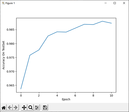
After 10 rounds, the average recognition accuracy on the training set reaches 98.88%, and the accuracy on the test set reaches 99%, of which the accuracy on the test set is shown in the figure below.

[1, 300]: loss: 0.820 , acc: 76.82 %
[1, 600]: loss: 0.237 , acc: 93.01 %
[1, 900]: loss: 0.152 , acc: 95.35 %
Accuracy on test set: 96.4 %
[2, 300]: loss: 0.126 , acc: 96.27 %
[2, 600]: loss: 0.109 , acc: 96.77 %
[2, 900]: loss: 0.094 , acc: 97.15 %
Accuracy on test set: 97.6 %
[3, 300]: loss: 0.084 , acc: 97.55 %
[3, 600]: loss: 0.080 , acc: 97.49 %
[3, 900]: loss: 0.075 , acc: 97.64 %
Accuracy on test set: 97.7 %
[4, 300]: loss: 0.072 , acc: 97.85 %
[4, 600]: loss: 0.066 , acc: 98.08 %
[4, 900]: loss: 0.060 , acc: 98.16 %
Accuracy on test set: 98.3 %
[5, 300]: loss: 0.058 , acc: 98.21 %
[5, 600]: loss: 0.060 , acc: 98.23 %
[5, 900]: loss: 0.055 , acc: 98.31 %
Accuracy on test set: 98.5 %
[6, 300]: loss: 0.047 , acc: 98.57 %
[6, 600]: loss: 0.054 , acc: 98.29 %
[6, 900]: loss: 0.053 , acc: 98.39 %
Accuracy on test set: 98.6 %
[7, 300]: loss: 0.048 , acc: 98.61 %
[7, 600]: loss: 0.044 , acc: 98.58 %
[7, 900]: loss: 0.049 , acc: 98.54 %
Accuracy on test set: 98.7 %
[8, 300]: loss: 0.045 , acc: 98.77 %
[8, 600]: loss: 0.043 , acc: 98.60 %
[8, 900]: loss: 0.043 , acc: 98.72 %
Accuracy on test set: 98.7 %
[9, 300]: loss: 0.040 , acc: 98.78 %
[9, 600]: loss: 0.037 , acc: 98.86 %
[9, 900]: loss: 0.042 , acc: 98.73 %
Accuracy on test set: 98.8 %
[10, 300]: loss: 0.038 , acc: 98.84 %
[10, 600]: loss: 0.034 , acc: 98.98 %
[10, 900]: loss: 0.037 , acc: 98.88 %
Accuracy on test set: 99.0 %

7, Complete code

import torch
import numpy as np
from matplotlib import pyplot as plt
from torch.utils.data import DataLoader
from torchvision import transforms
from torchvision import datasets
import torch.nn.functional as F

"""
Convolution operation use mnist Data sets, and 10-4，11 Similar, just here: 1.Output of training wheel acc 2.Use on Model torch.nn.Sequential
"""
# Super parameter ------------------------------------------------------------------------------------
batch_size = 64
learning_rate = 0.01
momentum = 0.5
EPOCH = 10

# Prepare dataset ------------------------------------------------------------------------------------
transform = transforms.Compose([transforms.ToTensor(), transforms.Normalize((0.1307,), (0.3081,))])
# softmax normalized exponential function( https://blog.csdn.net/lz_peter/article/details/84574716 ), where 0.1307 is the mean and 0.3081 is the std standard deviation

train_dataset = datasets.MNIST(root='./data/mnist', train=True, transform=transform)  # If there is no local, add download=True
test_dataset = datasets.MNIST(root='./data/mnist', train=False, transform=transform)  # train=True training set, = False test set
train_loader = DataLoader(train_dataset, batch_size=batch_size, shuffle=True)
test_loader = DataLoader(test_dataset, batch_size=batch_size, shuffle=False)

fig = plt.figure()
for i in range(12):
    plt.subplot(3, 4, i+1)
    plt.tight_layout()
    plt.imshow(train_dataset.train_data[i], cmap='gray', interpolation='none')
    plt.title("Labels: {}".format(train_dataset.train_labels[i]))
    plt.xticks([])
    plt.yticks([])
plt.show()


# The training set is out of order, and the test set is in order
# Design model using class ------------------------------------------------------------------------------
class Net(torch.nn.Module):
    def __init__(self):
        super(Net, self).__init__()
        self.conv1 = torch.nn.Sequential(
            torch.nn.Conv2d(1, 10, kernel_size=5),
            torch.nn.ReLU(),
            torch.nn.MaxPool2d(kernel_size=2),
        )
        self.conv2 = torch.nn.Sequential(
            torch.nn.Conv2d(10, 20, kernel_size=5),
            torch.nn.ReLU(),
            torch.nn.MaxPool2d(kernel_size=2),
        )
        self.fc = torch.nn.Sequential(
            torch.nn.Linear(320, 50),
            torch.nn.Linear(50, 10),
        )

    def forward(self, x):
        batch_size = x.size(0)
        x = self.conv1(x)  # One layer of convolution layer, one layer of pooling layer and one layer of activation layer (the figure shows convolution before activation and then pooling, with little difference)
        x = self.conv2(x)  # Once more
        x = x.view(batch_size, -1)  # The input required for flatten to become a fully connected network (batch, 20,4,4) = > (batch, 320), - 1 the automatic calculation here is 320
        x = self.fc(x)
        return x  # The last output is the dimension of 10, that is (corresponding to 0 ~ 9 of mathematical symbols)


model = Net()


# Construct loss and optimizer ------------------------------------------------------------------------------
criterion = torch.nn.CrossEntropyLoss()  # Cross entropy loss
optimizer = torch.optim.SGD(model.parameters(), lr=learning_rate, momentum=momentum)  # lr learning rate, momentum impulse


# Train and Test CLASS --------------------------------------------------------------------------------------
# Encapsulate a single round of a ring in a function class
def train(epoch):
    running_loss = 0.0  # This clears the loss of the entire epoch
    running_total = 0
    running_correct = 0
    for batch_idx, data in enumerate(train_loader, 0):
        inputs, target = data
        optimizer.zero_grad()

        # forward + backward + update
        outputs = model(inputs)
        loss = criterion(outputs, target)

        loss.backward()
        optimizer.step()

        # Add up the loss in operation to divide the following 300 times
        running_loss += loss.item()
        # Calculate the running accuracy acc
        _, predicted = torch.max(outputs.data, dim=1)
        running_total += inputs.shape[0]
        running_correct += (predicted == target).sum().item()

        if batch_idx % 300 == 299:  # Don't want to lose every time, waste time, choose an average loss every 300 times, and accuracy
            print('[%d, %5d]: loss: %.3f , acc: %.2f %%'
                  % (epoch + 1, batch_idx + 1, running_loss / 300, 100 * running_correct / running_total))
            running_loss = 0.0  # The loss of this small batch of 300 is cleared
            running_total = 0
            running_correct = 0  # This small batch of 300 acc is cleared

        # torch.save(model.state_dict(), './model_Mnist.pth')
        # torch.save(optimizer.state_dict(), './optimizer_Mnist.pth')


def test():
    correct = 0
    total = 0
    with torch.no_grad():  # Test sets do not count gradients
        for data in test_loader:
            images, labels = data
            outputs = model(images)
            _, predicted = torch.max(outputs.data, dim=1)  # dim = 1, column is the 0th dimension, and row is the 1st dimension. Find 1 along the row (1st dimension) Maximum and 2 Subscript of maximum value
            total += labels.size(0)  # Comparison operation between tensors
            correct += (predicted == labels).sum().item()
    acc = correct / total
    print('[%d / %d]: Accuracy on test set: %.1f %% ' % (epoch+1, EPOCH, 100 * acc))  # Find the accuracy of the test, correct number / total number
    return acc


# Start train and Test --------------------------------------------------------------------------------------
if __name__ == '__main__':
    acc_list_test = []
    for epoch in range(EPOCH):
        train(epoch)
        # if epoch % 10 == 9:  #Test once every 10 rounds of training
        acc_test = test()
        acc_list_test.append(acc_test)

    plt.plot(acc_list_test)
    plt.xlabel('Epoch')
    plt.ylabel('Accuracy On TestSet')
    plt.show()

reference material:
https://www.bilibili.com/video/BV1Y7411d7Ys?p=10