abstract
This example extracts some data from the plant seedling data set as the data set. The data set has 12 categories. It demonstrates how to use the mobile netv3 image classification model of pytorch version to realize the classification task.
Through this article, you can learn:
1. How to download from torchvision Models call mobilenetv3 model?
2. How do I customize how datasets are loaded?
3. How to use Cutout data enhancement?
4. How to use Mixup data enhancement.
5. How to achieve training and verification.
6. How to use cosine annealing to adjust the learning rate?
6. Two ways to write prediction.
Introduction to mobilenetv3
MobileNetV3 was proposed by google team in 2019. It is the third version of mobilenet series. Its parameters are obtained by NAS (network architecture search). In ImageNet classification tasks, compared with V2, the accuracy increases by 3.2% and the calculation delay decreases by 20%. Deep separable convolution is proposed in V1, and V2 adds Linear Bottleneck and Inverted Residual on the basis of V1. What are the characteristics of V3?
Let's take a look at the network structure of v3. There are two versions of V3: Large and Small, which are applicable to different scenarios respectively. The network structure is as follows:
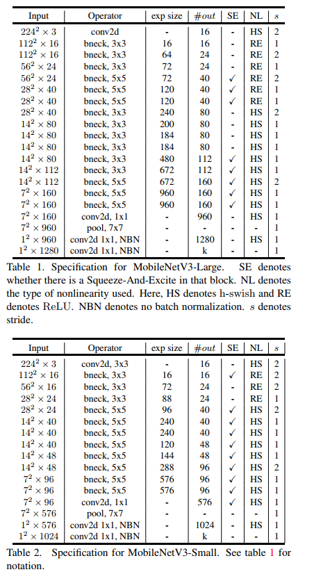
The above table shows the specific parameter settings, in which bneck is the basic structure of the network. SE represents whether channel attention mechanism is used. NL represents the type of activation function, including HS(h-swish),RE(ReLU). NBN means no BN operation. s means string. The network uses convolution string operation for downsampling instead of pooling operation.
Features of MobileNetV3:
- Inheriting the depth separable convolution of V1 and the residual structure with linear bottleneck of V2.
- The NetAdapt algorithm is used to obtain the optimal number of convolution cores and channels.
- A new activation function h-swish(x) is used to replace Relu6. Its formula is Relu6(x + 3)/6.
- The attention structure of Se channel is introduced, and Relu6(x + 3)/6 is used to approximate the sigmoid in SE module.
- The model is divided into Large and Small. In the ImageNet classification task, compared with V2, the Large accuracy rate increases by 3.2% and the calculation delay decreases by 20%.
MobileNetV3 code implementation (pytorch):
https://wanghao.blog.csdn.net/article/details/121607296
Data enhancement Cutout and Mixup
In order to improve my performance, I added two enhancement methods: Cutout and Mixup. To implement these two enhancements, you need to install torch toolbox. Installation command:
pip install torchtoolbox
Cutout is implemented in transforms.
from torchtoolbox.transform import Cutout

# Data preprocessing

transform = transforms.Compose([
    transforms.Resize((224, 224)),
    Cutout(),
    transforms.ToTensor(),
    transforms.Normalize([0.5, 0.5, 0.5], [0.5, 0.5, 0.5])

])
Mixup is implemented in the train method. Need to import package: from Torch toolbox tools import mixup_ data, mixup_ criterion
    for batch_idx, (data, target) in enumerate(train_loader):
        data, target = data.to(device, non_blocking=True), target.to(device, non_blocking=True)
        data, labels_a, labels_b, lam = mixup_data(data, target, alpha)
        optimizer.zero_grad()
        output = model(data)
        loss = mixup_criterion(criterion, output, labels_a, labels_b, lam)
        loss.backward()
        optimizer.step()
        print_loss = loss.data.item()
Project structure
MobileNetV3_demo
├─data
│  ├─test
│  └─train
│      ├─Black-grass
│      ├─Charlock
│      ├─Cleavers
│      ├─Common Chickweed
│      ├─Common wheat
│      ├─Fat Hen
│      ├─Loose Silky-bent
│      ├─Maize
│      ├─Scentless Mayweed
│      ├─Shepherds Purse
│      ├─Small-flowered Cranesbill
│      └─Sugar beet
├─dataset
│  └─dataset.py
├─train.py
├─test1.py
└─test.py
Import libraries used by the project
import torch.optim as optim
import torch
import torch.nn as nn
import torch.nn.parallel
import torch.utils.data
import torch.utils.data.distributed
import torchvision.transforms as transforms
from dataset.dataset import SeedlingData
from torch.autograd import Variable
from torchvision.models import mobilenet_v3_large
from torchtoolbox.tools import mixup_data, mixup_criterion
from torchtoolbox.transform import Cutout
Set global parameters
Set learning rate, BatchSize, epoch and other parameters to judge whether GPU exists in the environment. If not, use CPU. GPU is recommended. The CPU is too slow.
# Set global parameters
modellr = 1e-4
BATCH_SIZE = 16
EPOCHS = 300
DEVICE = torch.device('cuda' if torch.cuda.is_available() else 'cpu')
Image preprocessing and enhancement
Data processing is relatively simple. Cutout, Resize and normalization are added.
# Data preprocessing
transform = transforms.Compose([
    transforms.Resize((224, 224)),
    Cutout(),
    transforms.ToTensor(),
    transforms.Normalize([0.5, 0.5, 0.5], [0.5, 0.5, 0.5])

])
transform_test = transforms.Compose([
    transforms.Resize((224, 224)),
    transforms.ToTensor(),
    transforms.Normalize([0.5, 0.5, 0.5], [0.5, 0.5, 0.5])
])
Read data
Unzip the dataset and put it under the data folder, as shown in the figure:
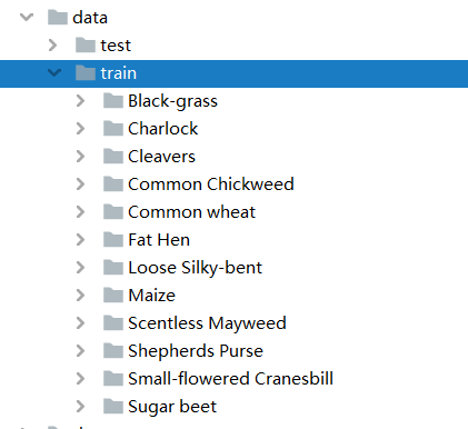
Then we create init. Net under the dataset folder Py and dataset Py, in datasets Py folder write the following code:
# coding:utf8
import os
from PIL import Image
from torch.utils import data
from torchvision import transforms as T
from sklearn.model_selection import train_test_split

Labels = {'Black-grass': 0, 'Charlock': 1, 'Cleavers': 2, 'Common Chickweed': 3,
          'Common wheat': 4, 'Fat Hen': 5, 'Loose Silky-bent': 6, 'Maize': 7, 'Scentless Mayweed': 8,
          'Shepherds Purse': 9, 'Small-flowered Cranesbill': 10, 'Sugar beet': 11}


class SeedlingData (data.Dataset):

    def __init__(self, root, transforms=None, train=True, test=False):
        """
        Main objective: to obtain the addresses of all pictures and divide the data according to training, verification and test
        """
        self.test = test
        self.transforms = transforms

        if self.test:
            imgs = [os.path.join(root, img) for img in os.listdir(root)]
            self.imgs = imgs
        else:
            imgs_labels = [os.path.join(root, img) for img in os.listdir(root)]
            imgs = []
            for imglable in imgs_labels:
                for imgname in os.listdir(imglable):
                    imgpath = os.path.join(imglable, imgname)
                    imgs.append(imgpath)
            trainval_files, val_files = train_test_split(imgs, test_size=0.3, random_state=42)
            if train:
                self.imgs = trainval_files
            else:
                self.imgs = val_files

    def __getitem__(self, index):
        """
        Return the data of one picture at a time
        """
        img_path = self.imgs[index]
        img_path=img_path.replace("\\",'/')
        if self.test:
            label = -1
        else:
            labelname = img_path.split('/')[-2]
            label = Labels[labelname]
        data = Image.open(img_path).convert('RGB')
        data = self.transforms(data)
        return data, label

    def __len__(self):
        return len(self.imgs)
Let's talk about the core logic of the code:
The first step is to establish a dictionary, define the ID corresponding to the category, and replace the category with numbers.
The second step is__ init__ Inside write the method to get the picture path. The test set has only one layer of path to read directly, and the training set is the category folder under the train folder. First obtain the category, and then obtain the specific image path. Then, using the method of segmenting data set in sklearn, the training set and verification set are segmented according to the ratio of 7:3.
The third step is__ getitem__ Method defines the method of reading a single picture and category. Since the image has a bit depth of 32 bits, I made a conversion when reading the image.
Then we were in train Py calls seedlingdata to read the data and remember to import the dataset just written py(from dataset.dataset import SeedlingData)
dataset_train = SeedlingData('data/train', transforms=transform, train=True)
dataset_test = SeedlingData("data/train", transforms=transform_test, train=False)
# Read data
print(dataset_train.imgs)

# Import data
train_loader = torch.utils.data.DataLoader(dataset_train, batch_size=BATCH_SIZE, shuffle=True)
test_loader = torch.utils.data.DataLoader(dataset_test, batch_size=BATCH_SIZE, shuffle=False)
Set model
- Set the loss function to NN CrossEntropyLoss().
- Set the model to mobilenet_v3_large, pre training set to true, num_classes is set to 12.
- The optimizer is set to adam.
- The learning rate adjustment strategy is cosine annealing.
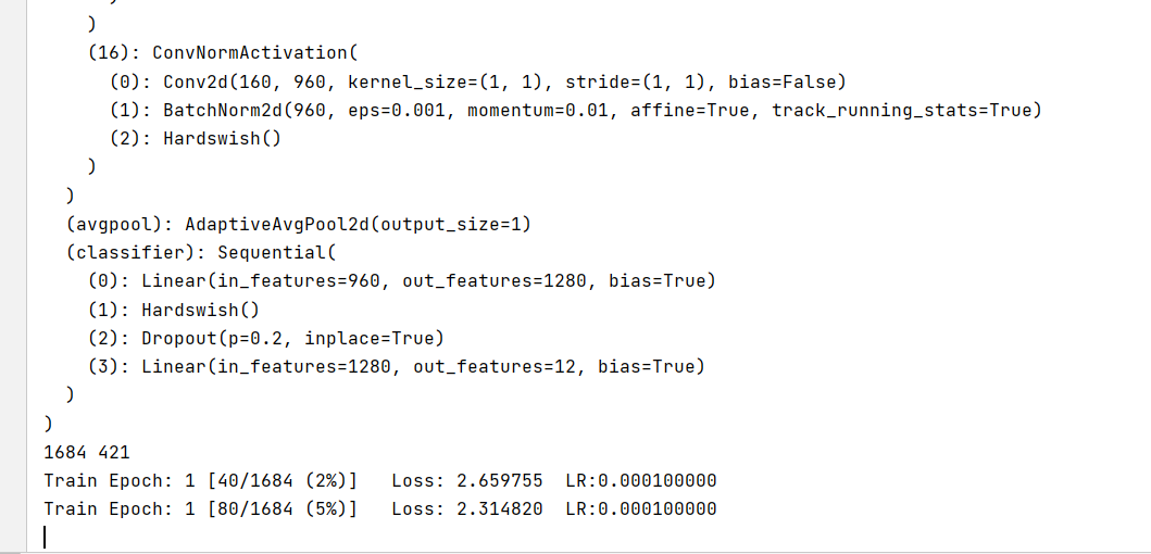
# Instantiate the model and move to GPU
criterion = nn.CrossEntropyLoss()
model_ft = mobilenet_v3_large(pretrained=True)
print(model_ft)
num_ftrs = model_ft.classifier[3].in_features
model_ft.classifier[3] = nn.Linear(num_ftrs, 12)
model_ft.to(DEVICE)
print(model_ft)
# Choose the simple and violent Adam optimizer and lower the learning rate
optimizer = optim.Adam(model_ft.parameters(), lr=modellr)
cosine_schedule = optim.lr_scheduler.CosineAnnealingLR(optimizer=optimizer,T_max=20,eta_min=1e-9)
Define training and verification functions
# Define training process
alpha=0.2
def train(model, device, train_loader, optimizer, epoch):
    model.train()
    sum_loss = 0
    total_num = len(train_loader.dataset)
    print(total_num, len(train_loader))
    for batch_idx, (data, target) in enumerate(train_loader):
        data, target = data.to(device, non_blocking=True), target.to(device, non_blocking=True)
        data, labels_a, labels_b, lam = mixup_data(data, target, alpha)
        optimizer.zero_grad()
        output = model(data)
        loss = mixup_criterion(criterion, output, labels_a, labels_b, lam)
        loss.backward()
        optimizer.step()
        lr = optimizer.state_dict()['param_groups'][0]['lr']
        print_loss = loss.data.item()
        sum_loss += print_loss
        if (batch_idx + 1) % 10 == 0:
            print('Train Epoch: {} [{}/{} ({:.0f}%)]\tLoss: {:.6f}\tLR:{:.9f}'.format(
                epoch, (batch_idx + 1) * len(data), len(train_loader.dataset),
                       100. * (batch_idx + 1) / len(train_loader), loss.item(),lr))
    ave_loss = sum_loss / len(train_loader)
    print('epoch:{},loss:{}'.format(epoch, ave_loss))

ACC=0
# Verification process
def val(model, device, test_loader):
    global ACC
    model.eval()
    test_loss = 0
    correct = 0
    total_num = len(test_loader.dataset)
    print(total_num, len(test_loader))
    with torch.no_grad():
        for data, target in test_loader:
            data, target = Variable(data).to(device), Variable(target).to(device)
            output = model(data)
            loss = criterion(output, target)
            _, pred = torch.max(output.data, 1)
            correct += torch.sum(pred == target)
            print_loss = loss.data.item()
            test_loss += print_loss
        correct = correct.data.item()
        acc = correct / total_num
        avgloss = test_loss / len(test_loader)
        print('\nVal set: Average loss: {:.4f}, Accuracy: {}/{} ({:.0f}%)\n'.format(
            avgloss, correct, len(test_loader.dataset), 100 * acc))
        if acc > ACC:
            torch.save(model_ft, 'model_' + str(epoch) + '_' + str(round(acc, 3)) + '.pth')
            ACC = acc


# train

for epoch in range(1, EPOCHS + 1):
    train(model_ft, DEVICE, train_loader, optimizer, epoch)
    cosine_schedule.step()
    val(model_ft, DEVICE, test_loader)
Operation results:
test
I introduce two common test methods. The first one is general. Manually load the data set and then make prediction. The specific operations are as follows:
The directory where the test set is stored is shown in the following figure:
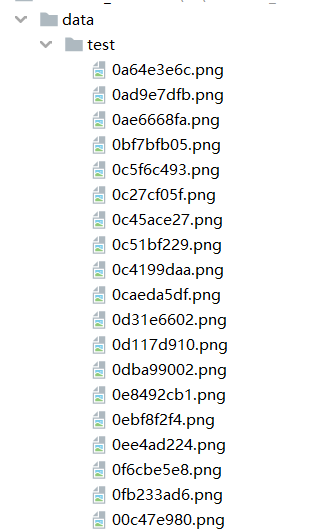
The first step is to define the category. The order of this category corresponds to the category order during training. Do not change the order!!!!
The second step is to define transforms, which is the same as the transforms of the verification set, without data enhancement.
Step 3: load the model and put it in DEVICE,
Step 4: read the picture and predict the category of the picture. Here, note that the Image of PIL library is used to read the picture. Don't use cv2. transforms doesn't support it.
import torch.utils.data.distributed
import torchvision.transforms as transforms
from PIL import Image
from torch.autograd import Variable
import os
classes = ('Black-grass', 'Charlock', 'Cleavers', 'Common Chickweed',
'Common wheat','Fat Hen', 'Loose Silky-bent',
'Maize','Scentless Mayweed','Shepherds Purse','Small-flowered Cranesbill','Sugar beet')
transform_test = transforms.Compose([
transforms.Resize((224, 224)),
transforms.ToTensor(),
transforms.Normalize([0.5, 0.5, 0.5], [0.5, 0.5, 0.5])
])
DEVICE = torch.device("cuda:0" if torch.cuda.is_available() else "cpu")
model = torch.load("model.pth")
model.eval()
model.to(DEVICE)
path='data/test/'
testList=os.listdir(path)
for file in testList:
img=Image.open(path+file)
img=transform_test(img)
img.unsqueeze_(0)
img = Variable(img).to(DEVICE)
out=model(img)
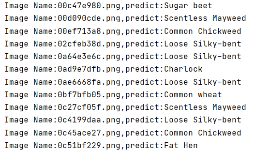
# Predict
_, pred = torch.max(out.data, 1)
print('Image Name:{},predict:{}'.format(file,classes[pred.data.item()]))
Operation results:
The second method uses a custom Dataset to read images
import torch.utils.data.distributed
import torchvision.transforms as transforms
from dataset.dataset import SeedlingData
from torch.autograd import Variable
classes = ('Black-grass', 'Charlock', 'Cleavers', 'Common Chickweed',
'Common wheat','Fat Hen', 'Loose Silky-bent',
'Maize','Scentless Mayweed','Shepherds Purse','Small-flowered Cranesbill','Sugar beet')
transform_test = transforms.Compose([
transforms.Resize((224, 224)),
transforms.ToTensor(),
transforms.Normalize([0.5, 0.5, 0.5], [0.5, 0.5, 0.5])
])
DEVICE = torch.device("cuda:0" if torch.cuda.is_available() else "cpu")
model = torch.load("model.pth")
model.eval()
model.to(DEVICE)
dataset_test =SeedlingData('data/test/', transform_test,test=True)
print(len(dataset_test))
# label of corresponding folder
for index in range(len(dataset_test)):
item = dataset_test[index]
img, label = item
img.unsqueeze_(0)
data = Variable(img).to(DEVICE)
output = model(data)
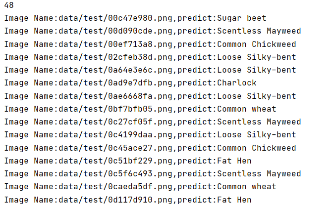
_, pred = torch.max(output.data, 1)
print('Image Name:{},predict:{}'.format(dataset_test.imgs[index], classes[pred.data.item()]))
index += 1
Operation results:
Full code: