1, Common skills in transfer learning: fine tuning

1.1 concept

1. Take the weights trained on the big data set as the initialization weight of the specific task (small data set), and retrain the network (modify the full connection layer output as needed); The training methods can be:
   1. Fine tune all layers;
   2. Fix the weights of the front layers of the network and only fine tune the back layers of the network for two reasons: A. avoid over fitting due to small amount of data; B. The features of the first few layers of CNN contain more general features (such as edge information, color information, etc.), which is very common for many tasks. However, the feature learning of the later layers of CNN focuses on high-level features, that is, semantic features, which is for data sets, and the semantic features of the later layers of different data sets are completely different;

1.2 steps

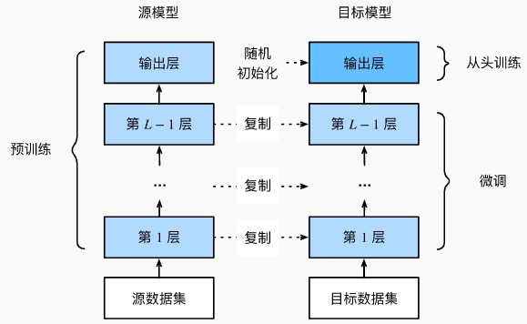
1. Train the neural network model on the source data set or save the model trained on the large data set, that is, the source model;
2. Create a new neural network model, namely target model. This copies all model designs on the source model (i.e. model layer design) and their parameters (except the output layer). It is assumed that the model parameters contain the knowledge learned from the source data set, which will also apply to the target data set;
3. To add an output layer to the target model, the number of output categories is the number of categories in the target data set, and then randomly initialize the model parameters of this layer;
4. The target model is trained on the target data set, the output layer is trained from scratch, and the parameters of all other layers will be fine tuned according to the parameters of the source model.

1.3 training

• The source data set is much more complex than the target data, and the fine-tuning effect is usually better;
• Usually use less learning rate and less data iteration;

1.4 realization

#Hot dog recognition
#Import the required package
from d2l import torch as d2l
from torch import nn
import torchvision
import torch
import os
%matplotlib inline

#Get dataset
"""
The hot dog dataset we use comes from the Internet. 
The dataset contains 1400 "positive" images of hot dogs and "negative" images of as many other foods as possible.
1000 images in two categories are used for training and the rest for testing.
"""
d2l.DATA_HUB['hotdog'] = (d2l.DATA_URL + 'hotdog.zip',
                         'fba480ffa8aa7e0febbb511d181409f899b9baa5')

data_dir = d2l.download_extract('hotdog')
print(data_dir)
#Output \data\hotdog

train_imgs=torchvision.datasets.ImageFolder(os.path.join(data_dir,'train'))
test_imgs=torchvision.datasets.ImageFolder(os.path.join(data_dir,'test'))
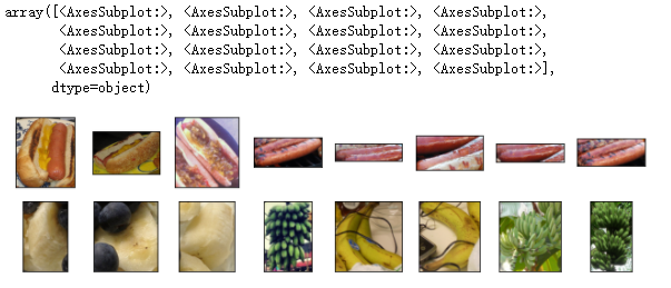
hotdogs=[train_imgs[i][0] for i in range(8)]
not_hotdogs=[train_imgs[-i-1][0] for i in range(8)]
d2l.show_images(hotdogs+not_hotdogs,2,8,scale=1.4)

# The mean and standard deviation of RGB channels are used to standardize each channel
"""
During training, we first cut the region with random size and random aspect ratio from the image, and then scale the region to\(224*224\)Enter the image. 
During the test, we scaled the height and width of the image to 256 pixels, and then cut the center\(224*224\)Area as input.
In addition, for RGB(Red, green and blue) color channels, we standardize each channel separately. 
Specifically, each value of the channel subtracts the average value of the channel, and then divides the result by the standard deviation of the channel.
"""
normalize=torchvision.transforms.Normalize([0.485,0.456,0.406],
                                           [0.229,0.224,0.225])
train_augs=torchvision.transforms.Compose([torchvision.transforms.RandomResizedCrop(224),#Cut randomly and resize to 224
                                          torchvision.transforms.RandomHorizontalFlip(),
                                          torchvision.transforms.ToTensor(),
                                          normalize])
test_augs=torchvision.transforms.Compose([torchvision.transforms.Resize(256),
                                          torchvision.transforms.CenterCrop(224),#Cut the picture from the center to 224 * 224
                                          torchvision.transforms.ToTensor(),
                                          normalize])

#We used ResNet-18 pre trained on ImageNet dataset as the source model. Here, we specify pre trained = true to automatically download the pre trained model parameters. 
#If you use this model for the first time, you need to connect to the Internet to download it.
pretrained_net=torchvision.models.resnet18(pretrained=True)

"""
The source model instance of pre training contains many feature layers and an output layer fc(Full connection layer).  
The main purpose of this division is to facilitate fine-tuning of model parameters of all layers except the output layer. 
The member variables of the source model are given below fc. 
"""
pretrained_net.fc
#output
#Linear(in_features=512, out_features=1000, bias=True)

finetune_net=torchvision.models.resnet18(pretrained=True)
finetune_net.fc=nn.Linear(finetune_net.fc.in_features,2)#The number of input neurons in the full connection layer is the characteristic number. Because it is classified as 2, the output is 2
nn.init.xavier_uniform_(finetune_net.fc.weight)#Random initialization of full connection layer weight
#Parameter containing:
tensor([[ 0.0378,  0.0630, -0.0080,  ..., -0.0220, -0.0511,  0.0959],
        [ 0.0556,  0.0227, -0.0262,  ..., -0.1059, -0.0171,  0.0051]],
       requires_grad=True)

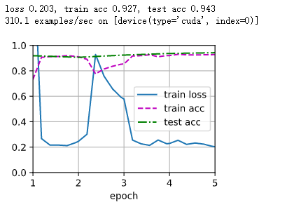
#Fine tuning model
# If param_group=True, the model parameters in the output layer will use ten times the learning rate
def train_fine_tuning(net, learning_rate, batch_size=128, num_epochs=5,
                      param_group=True):
    train_iter = torch.utils.data.DataLoader(torchvision.datasets.ImageFolder(
        os.path.join(data_dir, 'train'), transform=train_augs),
        batch_size=batch_size, shuffle=True)
    test_iter = torch.utils.data.DataLoader(torchvision.datasets.ImageFolder(
        os.path.join(data_dir, 'test'), transform=test_augs),
        batch_size=batch_size)
    devices = d2l.try_all_gpus()
    loss = nn.CrossEntropyLoss(reduction="none")
    if param_group:
        params_1x = [param for name, param in net.named_parameters()
             if name not in ["fc.weight", "fc.bias"]]
        trainer = torch.optim.SGD([{'params': params_1x},
                                   {'params': net.fc.parameters(),
                                    'lr': learning_rate * 10}],
                                lr=learning_rate, weight_decay=0.001)
    else:
        trainer = torch.optim.SGD(net.parameters(), lr=learning_rate,
                                  weight_decay=0.001)
    d2l.train_ch13(net, train_iter, test_iter, loss, trainer, num_epochs,
                   devices)
train_fine_tuning(finetune_net, 5e-5)                  

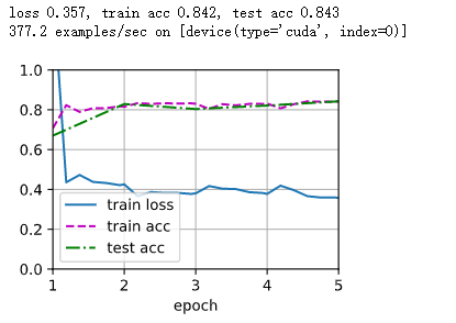
#For comparison, we define the same model, but initialize all its model parameters to random values. 
#Since the whole model needs to be trained from scratch, we need to use a larger learning rate.
scratch_net = torchvision.models.resnet18()
scratch_net.fc = nn.Linear(scratch_net.fc.in_features, 2)
train_fine_tuning(scratch_net, 5e-4, param_group=False)

• Reference website: https://zh-v2.d2l.ai/chapter_computer-vision/fine-tuning.html