Previous articles in this column have discussed that under the condition of complex and changeable exogenous stimuli, the structure of time series data will change, so that outdated data is no longer suitable for current time series modeling. The general time series econometric modeling method itself does not have the function of identifying structural change parameters and change time points; The commonly used structural stability measurement and test methods also need more manual intervention or computational resource investment, which is particularly prominent when dealing with a large number of time series modeling requirements. In order to solve the structural change problem encountered when dealing with a large number of time series modeling requirements in the process of quantitative R & D, I have pondered a series of modeling methods to deal with the structural change of time series, which are respectively suitable for time series analysis in different scenarios. This issue introduces the first requirement scenario and its modeling method.

Scene description

(1) It is necessary to sensitively identify the current trend state of the time series, that is, to sensitively identify the current n-order differential positive and negative bias of the time series

(2) The determination of the current trend state of time series needs sufficient time step data for verification

(3) Distinguish between the clear part of the trend and the fuzzy part of the trend

(4) The future estimation of time series only considers the latest information in line with the current trend

(5) Hold a conservative attitude towards data mutations that are not verified by sufficient time step data

(6) Conduct hypothesis test on the fuzzy part of the trend to determine the trend state

(7) The environment is changeable, the data is sparse, and the data samples in the same period often fail to meet the needs of parameter estimation of classical measurement methods

Modeling method

According to the above scenarios, research the modeling method to meet the requirements:

The first step is to calculate the n-order difference sequence of the time series according to the demand of point (1). Because in the process of practical application, the trend change of time series is generally dominated by linear change (such as the research case of historical data of income statement of previous listed companies). Except for random change, the deviation of difference series mostly occurs in order 1 and 2, and there is rarely difference deviation above order 3. Therefore, the modeling method in this period analyzes the current trend state of the time series according to the positive and negative bias of the first-order and second-order difference series of the time series, that is, calculates and analyzes the time series First order differenceAnd second order difference .

The second step is to set the minimum time step MS required to determine the current trend state of the time series according to the demand of point (2), that is, the minimum data sample size continuous with the latest time point data.

In the third step, according to the requirements of points (3) and (4), from the first-order differenceStart backtracking at the latest time point of:

(a) IfAll greater than 0,

And ，

And( or )，

Then it is determined that the current trend state level 1 is clearly positive (+), andIs the first-order sequence of current trend state;

(b) IfAll less than 0,

And ，

And( or )，

Then it is determined that the current trend state level 1 is clearly negative (-), andIs the first-order sequence of current trend state;

(c) If Both greater than 0 and less than 0,

And，

And does not existMake( All greater than 0 or all less than 0),

And[Or( )All greater than 0 or all less than 0)],

Then the current trend state level 1 is undetermined, andIs the first-order sequence of current trend state;

(d) Meet the requirements of point (5), ifAnd ，

And does not existMake( All greater than 0 or all less than 0),

And[Or( )All greater than 0 or all less than 0)],

Then the current trend state of order 1 is none (n), andIt is the first-order sequence of the current trend state.

Step 4: in addition to the case that the first-order state of the current trend state is none, further analyze the first-order state of the current trend state and the first-order sequence of the current trend state:

(a) Meet the requirements of point (6). If the current trend state is of order 1 to be determined, the current trend state will be of order 1 sequenceBy significance level The one tailed hypothesis tests biased to positive and negative are conducted respectively, and finally it is determined that the first order of the current trend state is positive (+), negative (-) or none (n). The second-order difference is no longer performed analysis.

(b) If the first order of the current trend state is clearly positive (+) or negative (-), the second-order difference Carry out the same analysis steps to identify the second-order state of the current trend state and the second-order sequence of the current trend state. But the third-order difference is no longer carried out analysis.

By the end of step 4, the requirements of point (1) (2) (3) (5) (6) have been solved, and the current trend structure of time series - that is, the identification of current trend status and current trend series has been completed. The modeler can combine the identification results with the commonly used parameter estimation methods for subsequent work, or perform parameter estimation according to the next steps.

Step 5: meet the requirements of points (4) and (7), and establish the following time series deduction model (prediction model):

(a) If the 2nd order of the current trend state is positive (+) or negative (-), calculate the 2nd order sequence of the current trend stateThe mean value of is the second-order change value G, and the latest value of the first-order difference is takenIs the first-order change value D, and the latest value of the time series is taken Is the base period value A. Taking A, D and G as the parameters of the time series deduction model, the base period , the calculation formula of the future deduction sequence (prediction sequence) of the model is:

(b) The 1st order of the current trend state is positive (+) or negative (-), and the 1st order sequence of the current trend state is calculated The mean value of is the first-order change value D, and the latest value of the time series is taken Is the base period value A. Take A and D as the parameters of the time series deduction model, and the base period , the calculation formula of the future deduction sequence (prediction sequence) of the model is:

(c) The current trend state of order 1 is none (n), and the latest value of the time series is takenIs the base period value A. Taking A as the time series deduction model parameter, the calculation formula of the future deduction series (prediction Series) of the model is:

In order to facilitate memory and distinguish from the modeling method introduced later, this method is called Strict Latest Status Model, which can be directly implemented by using Python library valuequant. The analyst can execute the command pip install valuequant on the terminal to install the module.

Simple examples of code implementation and practical application

Firstly, a time series with trend structure change is constructed as a simple test sequence.

>>> #Create a simple test sequence 
>>> import numpy as np 
>>> import pandas as pd 
>>> series=pd.Series(np.arange(1,13)+1+np.random.normal(0,0.1,12),index=pd.date_range(start='2010-01-01',periods=12,freq='Q-DEC')) 
>>> aseries=pd.Series(series[-1]+np.random.normal(0,0.1,12),index=pd.date_range(start='2013-01-01',periods=12,freq='Q-DEC')) 
>>> series=pd.concat((series,aseries)) 
>>> aseries=pd.Series(np.arange(1,21)*1.2+series[-1]+np.random.normal(0,0.1,20),index=pd.date_range(start='2016-01-01',periods=20,freq='Q-DEC')) 
>>> series=pd.concat((series,aseries)) 
>>> #Graphic visual demonstration of time series form 
>>> plt.plot(series) 
>>> plt.show()

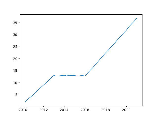
As shown in the figure above, there are two trend structure changes in the test time series. Next, valuequant implements the current trend structure - that is, the identification and parameter estimation of the current trend state and current trend sequence.

>>> #Call valuequant and log in the account. The login account can be https://www.boomevolve.com Register to obtain 
>>> import valuequant as vq 
>>> vq.login(name=<title of account>,pswd=<Account password>) Login succeeded 
>>> #The minstep parameter is the minimum time step required to determine the current trend state of the time series, and the significance parameter is the significance level of the hypothesis test 
>>> model=vq.Models.strict_latest_status_model(series=series,minstep=8,significance=0.3) 
>>> #Get modeling results 
>>> model.model() 
{'method': 'l1', 'step': 21, 'params': {'l1_diff': 1.201133, 'value_latest': 36.725542}, 'status': {'l1': '+', 'l2': 'n'}} 
>>> #The results show that the current trend state status is first-order positive, second-order none, and the current trend state sequence is the last 21 steps. The first-order change value is used to deduce the future sequence 
>>> #You can use model Fit() command to obtain the fitting data in the sample, and use model Forecast (t = < steps to be predicted >) obtains extrapolation data outside the sample 
>>> #Drawing display results 
>>> plt.plot(model.data()) 
>>> plt.plot(model.fit()) 
>>> plt.plot(model.forecast(t=12)) 
>>> plt.show()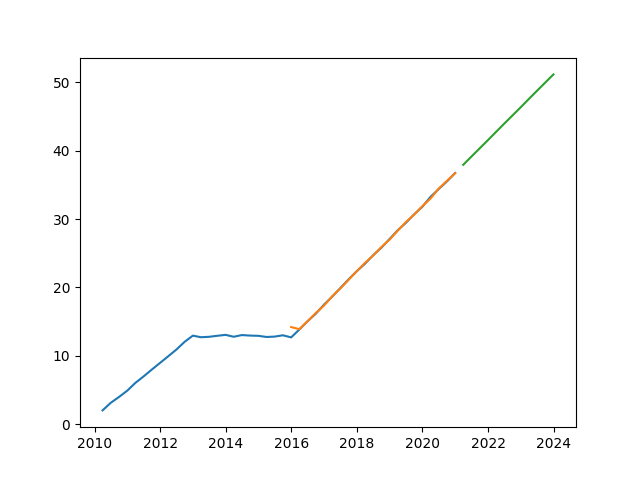

The above is a simple code implementation of Strict Latest Status Model.

Note: valuequant will automatically filter abnormal samples during modeling. Analysts can also add more exception handling processes before use according to modeling needs.

Application example of time series with seasonal items

The main function of this method is to identify the trend structure changes of time series. For time series containing seasonal items, it is necessary to decompose the seasonal items of time series first. This requirement can be met by setting the seasonal parameter of the valuequant related model. Based on the above test time series, the seasonal multiplier is added to construct the test series with seasonal items for demonstration.

>>> #Build test sequence with seasonal items 
>>> series=series*pd.Series(np.tile([1.05,1.1,0.95,0.9],int(np.ceil(len(series)/4)))[:len(series)], index=series.index) 
>>> #Drawing demonstration test sequence 
>>> plt.plot(series) 
>>> plt.show() 
>>> set up seasonal=True(Default to False)，Separating time series seasonal terms 
>>> model=vq.Models.strict_latest_status_model(series=series,minstep=8,significance=0.3,seasonal=True) 
>>> model.model() 
{'method': 'l1', 'step': 22, 'params': {'l1_diff': 1.19459, 'value_latest': 37.077803}, 'status': {'l1': '+', 'l2': 'n'}, 'seasonal': {'12': 0.899668, '3': 1.049939, '6': 1.099923, '9': 0.949162}, 'qorder': ['3', '6', '9', '12']} 
>>> #The model results add an estimate of the seasonal multiplier 'seasonal' 
>>> #The drawing shows the modeling results 
>>> plt.plot(model.data()) 
>>> plt.plot(model.fit()) 
>>> plt.plot(model.forecast(t=12)) 
>>> plt.show()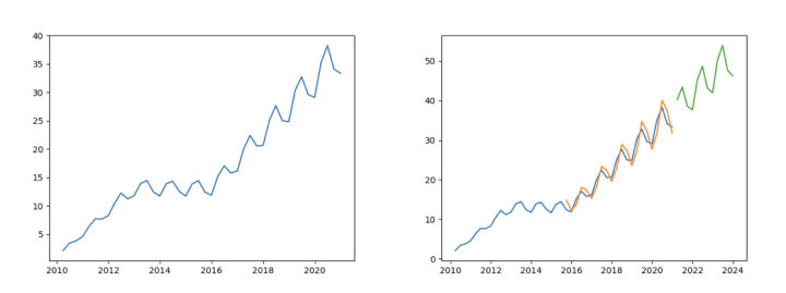

​

Parameter mutation problem and practical treatment method

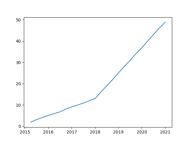
It should be noted that this method does not provide the function of direct identification in the case of parameter mutation. A test sequence with parameter mutation but constant trend direction is constructed for illustration.

>>> #Construct a test sequence with abrupt parameters but constant trend direction 
>>> series=pd.Series(np.arange(1,13)+1+np.random.normal(0,0.1,12),index=pd.date_range(start='2015-01-01',periods=12,freq='Q-DEC')) 
>>> aseries=pd.Series(np.arange(1,13)*3+series[-1]+np.random.normal(0,0.1,12),index=pd.date_range(start='2018-01-01',periods=12,freq='Q-DEC')) 
>>> series=pd.concat((series,aseries)) 
>>> plt.plot(series) 
>>> plt.show()

​>>> # Set the annual parameter and use the time weight in hypothesis test and mean calculation 
>>> model=vq.Models.strict_latest_status_model(series=series,minstep=8,significance=0.3,anneal=0.9) 
>>> model.model() 
{'method': 'l1', 'step': 24, 'params': {'l1_diff': 2.564423, 'value_latest': 48.890396}, 'status': {'l1': '+', 'l2': 'n'}}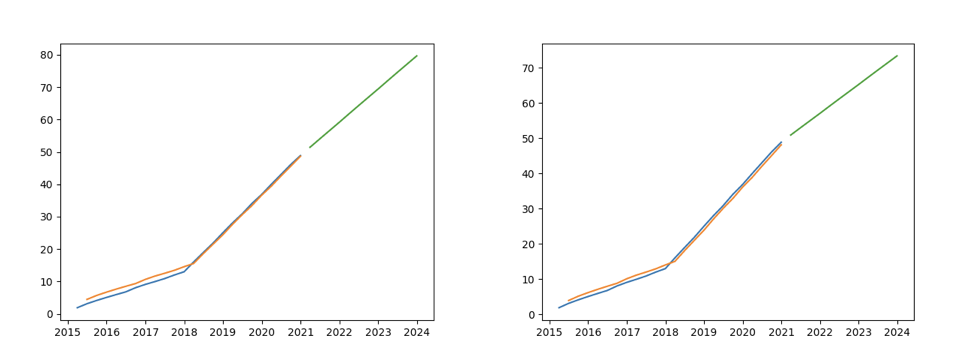

The above figure on the left shows the modeling example with anneal=0.9, and the figure on the right shows the modeling example without anneal. It can be intuitively observed that the model parameter estimation with anneal tends to the time series characteristics after parameter mutation. However, the problem of parameter mutation can not be completely solved.

Using conservative estimation parameters

In addition, because the strict state update model is based on the estimation of the change value of the first-order and second-order difference, when the first-order difference direction is inconsistent with the second-order difference direction, the future deduction sequence (prediction sequence) of the model will reverse the first-order difference direction within a limited number of steps. If the analyst is conservative about the reversal, the parameter conservative=True (False by default) of the valuequant correlation model can be set so that the model no longer uses the second-order change value, but uses the first-order difference change rate g, and the calculation formula of the future deduction sequence (prediction sequence) of the model is changed to

The specific code is as follows:

>>> #A sequence with second-order variation and inconsistent first-order and second-order difference directions is constructed 
>>> series=pd.Series(8-6*pow(0.9,np.arange(1,13))+np.random.normal(0,0.001,12),index=pd.date_range(start='2018-01-01',periods=12,freq='Q-DEC')) 
>>> #Set the strict status update model parameter conservative=True 
>>> model=vq.Models.strict_latest_status_model(series=series,minstep=8,significance=0.3,conservative=True) 
>>> model.model() 
{'method': 'l2smooth', 'step': 12, 'params': {'l1_latest': 0.18683799999999984, 'value_latest': 6.304831, 'l2smooth_rate': 1.0}, 'status': {'l1': '+', 'l2': '-'}, 'smooth': True} 
>>> #Drawing display results 
>>> plt.plot(model.data()) 
>>> plt.plot(model.fit()) 
>>> plt.plot(model.forecast(t=12)) 
>>> plt.show()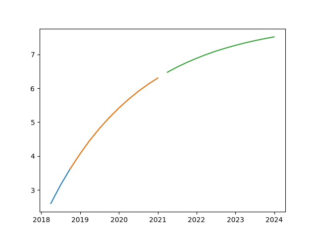

This can make the absolute value of the first-order difference of the future deduction sequence tend to 0 instead of direction reversal.

Limitations of Strict Latest Status Model

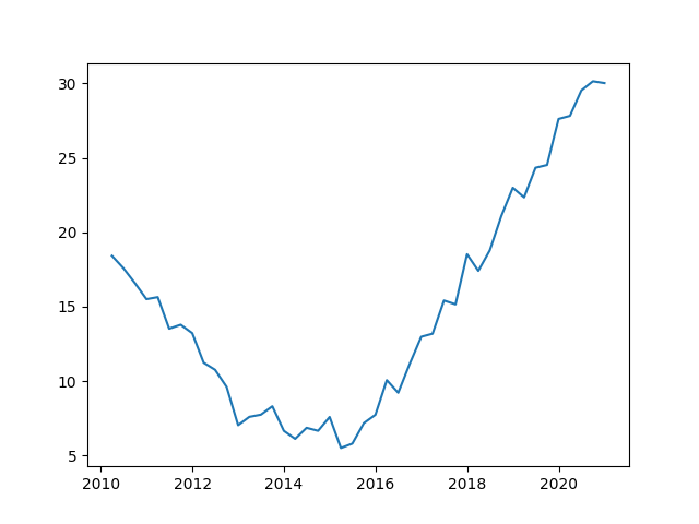
Limitation 1: the model is not suitable for time series with large fluctuation range, and subtle trend structure changes are easy to be covered up by fluctuations. As shown in the following figure, the trend structure of time series has actually changed many times, but due to large fluctuations, the model will classify it into the same band and only conduct hypothesis test once.

​

>>> #Build test sequence 
>>> series=pd.Series(20-np.arange(1,13)+np.random.normal(0,1,12),index=pd.date_range(start='2010-01-01',periods=12,freq='Q-DEC')) 
>>> aseries=pd.Series(series[-1]+np.random.normal(0,1,12),index=pd.date_range(start='2013-01-01',periods=12,freq='Q-DEC')) 
>>> series=pd.concat((series,aseries)) 
>>> aseries=pd.Series(np.arange(1,21)*1.2+series[-1]+np.random.normal(0,1,20),index=pd.date_range(start='2016-01-01',periods=20,freq='Q-DEC')) 
>>> series=pd.concat((series,aseries)) 
>>> #Build a strict status update model 
>>> model=vq.Models.strict_latest_status_model(series=series,minstep=8,significance=0.3) 
>>> model.model() 
{'method': 'random', 'step': 44, 'params': {'value_mean': 14.749896}, 'status': {'l1': 'n'}} 
>>> #The results show that this method classifies the whole time series into the same trend blurred band without identifying the actual change of trend structure

Limitation 2: when dealing with the time series with multiplier seasonal term and high-order difference change at the same time, the inevitable error caused by separating the multiplier of seasonal term is easy to lead to the problem of heteroscedasticity, which will affect the trend state identification after separating the seasonal term.

>>> #Constructing second-order trend series 
>>> trends=pd.Series(pow(np.arange(1, 40 + 1),2)*(-0.1)+np.arange(1, 40 + 1) * 10 +10 + np.random.normal(0, 0.01, 40), index=pd.date_range(start='2012-03-31',freq='Q-DEC',periods=40)) 
>>> #The strict state update model of second-order trend sequence is constructed 
>>> tmodel=vq.Models.strict_latest_status_model(series=trends,minstep=8,significance=0.3) 
>>> tmodel.model() 
{'method': 'l2', 'step': 40, 'params': {'l2_diff': -0.200825, 'l1_latest': 2.0771250000000236, 'value_latest': 249.980014}, 'status': {'l1': '+', 'l2': '-'}} 
>>> #Based on the above trend series, seasonal items are added for comparison 
>>> series=trends*pd.Series(np.tile([1.05,1.1,0.95,0.9],int(np.ceil(len(series)/4)))[:len(series)], index=series.index) 
>>> model=vq.Models.strict_latest_status_model(series=series,minstep=8,significance=0.3,seasonal=True) 
>>> model.model() 
{'method': 'l1', 'step': 40, 'params': {'l1_diff': 5.899722, 'value_latest': 250.011994}, 'status': {'l1': '+', 'l2': 'n'}, 'seasonal': {'12': 0.899885, '3': 1.048498, '6': 1.102457, '9': 0.953143}, 'qorder': ['3', '6', '9', '12']} 
>>> #Comparing the two modeling results, the strict state update model can not identify the second-order change of trend after adding seasonal items 
>>> plt.plot(tmodel.data()) 
>>> plt.plot(tmodel.fit()) 
>>> plt.plot(tmodel.forecast(12)) 
>>> plt.show() 
>>> plt.plot(model.data()) 
>>> plt.plot(model.fit()) 
>>> plt.plot(model.forecast(12)) 
>>> plt.show()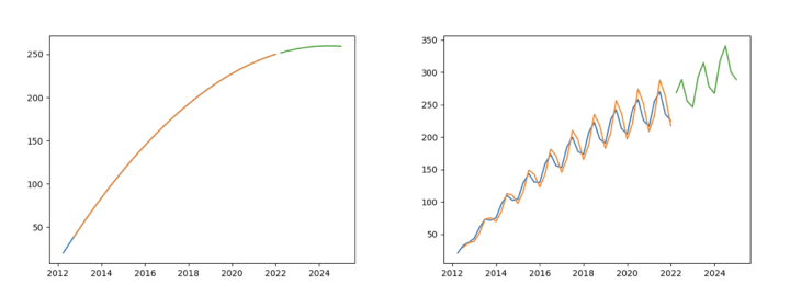

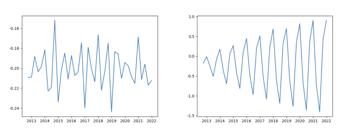
As shown in the left figure above, the model can identify the second-order change of time series without multiplier seasonal term; However, as shown in the figure on the right above, the test is carried out after the time series is multiplied by the seasonal term. At this time, only the first-order change of the time series can be identified. Next, analyze the data characteristics of the original trend series and the series containing seasonal items, and find out the reasons.

>>> #Calculate the value sequence of the sequence containing seasonal items after separating and estimating the seasonal items 
>>> pseries=series/pd.Series(np.tile([1.048498,1.102457,0.953143,0.899885],int(np.ceil(len(series)/4)))[:len(series)], index=series.index) 
>>> #Comparing the original trend series with the series containing seasonal items, the first-order difference series and the second-order difference series of the series after the seasonal items are separated and estimated 
>>> plt.plot(trends.diff()) 
>>> plt.show() 
>>> plt.plot(pseries.diff()) 
>>> plt.show() 
>>> plt.plot(trends.diff().diff()) 
>>> plt.show() 
>>> plt.plot(pseries.diff().diff()) 
>>> plt.show()

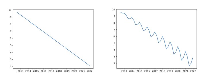
Compared with the first-order difference of the trend sequence in the left figure above, the right figure contains the first-order difference of the sequence after the seasonal term sequence is separated and estimated. In the right figure, there are still errors caused by seasonal fluctuations after the seasonal term is separated.

Then compare the second-order difference of the trend sequence in the left figure and the second-order difference of the sequence with seasonal items in the right figure. The right figure shows obvious heteroscedasticity. Therefore, when there is an error in the separation of seasonal terms, the model is prone to high-order misjudgment.

Limitation 3: it is easy to ignore the long-term trend direction.

>>> #Construct a long-term cycle sequence for elaboration 
>>> series=pd.Series(np.tile(np.append(np.linspace(10,1,10),np.linspace(0,9,10)),4)+np.random.normal(0, 0.2, 80), index=pd.date_range(start='2001-01-01',periods=80,freq='Q-DEC')) 
>>> #Build a strict status update model 
>>> model=vq.Models.strict_latest_status_model(series=series,minstep=8,significance=0.3) 
>>> model.model() 
{'method': 'l1', 'step': 10, 'params': {'l1_diff': 0.991741, 'value_latest': 9.284276}, 'status': {'l1': '+', 'l2': 'n'}} 
>>> #According to the above results, the model misjudges that the time series is a first-order growth series 
>>> plt.plot(model.data()) 
>>> plt.plot(model.fit()) 
>>> plt.plot(model.forecast(12)) 
>>> plt.show()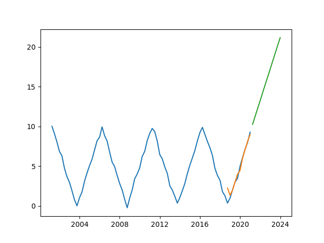

As shown in the figure above, the model only recognizes part of the short-term bands of the time series, but ignores the long-term law.

Limitation 4: as mentioned above, the model can not directly identify parameter mutation.

If analysts need to solve the above problems or deal with different demand scenarios from the model, please read the introduction of other relevant modeling methods in the subsequent articles of this column.