API . Training neural network needs many steps. You need to specify how to input training data, initialize model parameters, perform forward and backward transfers in the network, update weights based on calculated gradients, perform model checkpoints, and so on. Most of these steps will eventually be repeated during the forecast process. For novices and experienced developers, all of these are daunting.
Fortunately, MXNet modularizes common code for training and reasoning in the module package. Module provides advanced and intermediate interfaces for executing predefined networks. Both interfaces can be used interchangeably. In this tutorial, we'll show you how to use these two interfaces.
Preliminary
The first is a primary usage demo:
import logging
import random
logging.getLogger().setLevel(logging.INFO)

import mxnet as mx
import numpy as np

mx.random.seed(1234)
np.random.seed(1234)
random.seed(1234)

fname = mx.test_utils.download('https://s3.us-east-2.amazonaws.com/mxnet-public/letter_recognition/letter-recognition.data')
data = np.genfromtxt(fname, delimiter=',')[:,1:]
label = np.array([ord(l.split(',')[0])-ord('A') for l in open(fname, 'r')])

batch_size = 32
ntrain = int(data.shape[0]*0.8)
train_iter = mx.io.NDArrayIter(data[:ntrain, :], label[:ntrain], batch_size, shuffle=True)
val_iter = mx.io.NDArrayIter(data[ntrain:, :], label[ntrain:], batch_size)
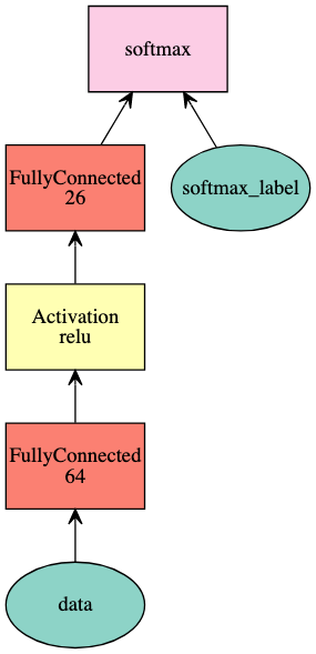
Network definition, using Symbol:
net = mx.sym.Variable('data')
net = mx.sym.FullyConnected(net, name='fc1', num_hidden=64)
net = mx.sym.Activation(net, name='relu1', act_type="relu")
net = mx.sym.FullyConnected(net, name='fc2', num_hidden=26)
net = mx.sym.SoftmaxOutput(net, name='softmax')
mx.viz.plot_network(net, node_attrs={"shape":"oval","fixedsize":"false"})
Creating a Module
Module class is used to introduce modules, which can be built by specifying the following parameters:
- symbol: network definition
- context: device (or device list) for execution
- data_names: enter a list of data variable names
- label_names: enter a list of label variable names
For the net defined above, there is only one data named data, and only one label is automatically named softmax_label, this is based on our name softmax in softmax output.
mod = mx.mod.Module(symbol=net,
                    context=mx.cpu(),
                    data_names=['data'],
                    label_names=['softmax_label'])
Intermediate-level Interface
We have created the module. Now let's look at how to run training and reasoning using the module's intermediate api. These APIs enable developers to flexibly perform step-by-step calculations by running forward and backward. It is also useful for debugging. In order to train a module, the following steps need to be implemented:
- bind: prepare the environment for computing by allocating memory.
- init_params: assign and initialize parameters.
- init_optimizer: initializes the optimizer. The default is sgd.
- metric.create : creates a calculated measure from the input measure name.
- Forward: forward calculation.
- update_metric: the calculated metric that calculates and accumulates the output of the last forward calculation.
- Backward: backward calculation.
- update: updates the parameters based on the installed optimizer and the gradient calculated in the previous previous pre post batch.
The specific implementation is as follows:
# allocate memory given the input data and label shapes
mod.bind(data_shapes=train_iter.provide_data, label_shapes=train_iter.provide_label)
# initialize parameters by uniform random numbers
mod.init_params(initializer=mx.init.Uniform(scale=.1))      # mxnet.initializer
# use SGD with learning rate 0.1 to train
mod.init_optimizer(optimizer='sgd', optimizer_params=(('learning_rate', 0.1), ))   # mxnet.optimiazer
# use accuracy as the metric
metric = mx.metric.create('acc')       # mxnet.mxtric
# train 5 epochs, i.e. going over the data iter one pass
for epoch in range(5):
    train_iter.reset()       # Re iteration
    metric.reset()           # Reassessment
    for batch in train_iter:
        mod.forward(batch, is_train=True)       # compute predictions   Forward
        mod.update_metric(metric, batch.label)  # accumulate prediction accuracy   Calculate evaluation index
        mod.backward()                          # compute gradients     # reverse
        mod.update()                            # update parameters     # Update parameters
    print('Epoch %d, Training %s' % (epoch, metric.get()))
be careful module.bind and symbol.bind dissimilarity.
Note: there are many abbreviations in mxnet: mx.symbol=mx.sys; mx.initializer=mx.init; mx.module=mx.mod
Epoch 0, Training ('accuracy', 0.434625)
Epoch 1, Training ('accuracy', 0.6516875)
Epoch 2, Training ('accuracy', 0.6968125)
Epoch 3, Training ('accuracy', 0.7273125)
Epoch 4, Training ('accuracy', 0.7575625)
High-level Interface
In the previous section, intermediate API is used, so there are many steps. In this section, advanced API is used fit Function.
1. Training
# reset train_iter to the beginning   Reset iterator
train_iter.reset()

# create a module
mod = mx.mod.Module(symbol=net,        # Create module
                    context=mx.cpu(),
                    data_names=['data'],
                    label_names=['softmax_label'])

# fit the module         # train
mod.fit(train_iter,
        eval_data=val_iter,
        optimizer='sgd',
        optimizer_params={'learning_rate':0.1},
        eval_metric='acc',
        num_epoch=7)
INFO:root:Epoch[0] Train-accuracy=0.325437
INFO:root:Epoch[0] Time cost=0.550
INFO:root:Epoch[0] Validation-accuracy=0.568500
INFO:root:Epoch[1] Train-accuracy=0.622188
INFO:root:Epoch[1] Time cost=0.552
INFO:root:Epoch[1] Validation-accuracy=0.656500
INFO:root:Epoch[2] Train-accuracy=0.694375
INFO:root:Epoch[2] Time cost=0.566
INFO:root:Epoch[2] Validation-accuracy=0.703500
INFO:root:Epoch[3] Train-accuracy=0.732187
INFO:root:Epoch[3] Time cost=0.562
INFO:root:Epoch[3] Validation-accuracy=0.748750
INFO:root:Epoch[4] Train-accuracy=0.755375
INFO:root:Epoch[4] Time cost=0.484
INFO:root:Epoch[4] Validation-accuracy=0.761500
INFO:root:Epoch[5] Train-accuracy=0.773188
INFO:root:Epoch[5] Time cost=0.383
INFO:root:Epoch[5] Validation-accuracy=0.715000
INFO:root:Epoch[6] Train-accuracy=0.794687
INFO:root:Epoch[6] Time cost=0.378
INFO:root:Epoch[6] Validation-accuracy=0.802250
By default, the parameters in fit are as follows:
eval_metric set to accuracy, optimizer to sgd and optimizer_params to (('learning_rate', 0.01),).
y = mod.predict(val_iter)
assert y.shape == (4000, 26)
Sometimes we don't care about the specific prediction value, just want to know the indicators on the test set, then we can call the score() function to achieve. It will be evaluated based on the metric you provide:
score = mod.score(val_iter, ['acc'])
print("Accuracy score is %f" % (score[0][1]))
assert score[0][1] > 0.76, "Achieved accuracy (%f) is less than expected (0.76)" % score[0][1]
Accuracy score is 0.802250
Of course, other indicators can also be used: top_k_acc(top-k-accuracy), F1, RMSE, MSE, MAE, ce(CrossEntropy). For more indicators, see Evaluation metric.
# construct a callback function to save checkpoints
model_prefix = 'mx_mlp'
checkpoint = mx.callback.do_checkpoint(model_prefix)

mod = mx.mod.Module(symbol=net)
mod.fit(train_iter, num_epoch=5, epoch_end_callback=checkpoint)    # Write to epoch_ end_ Every epoch in the callback will be saved once
INFO:root:Epoch[0] Train-accuracy=0.098437
INFO:root:Epoch[0] Time cost=0.421
INFO:root:Saved checkpoint to "mx_mlp-0001.params"
INFO:root:Epoch[1] Train-accuracy=0.257437
INFO:root:Epoch[1] Time cost=0.520
INFO:root:Saved checkpoint to "mx_mlp-0002.params"
INFO:root:Epoch[2] Train-accuracy=0.457250
INFO:root:Epoch[2] Time cost=0.562
INFO:root:Saved checkpoint to "mx_mlp-0003.params"
INFO:root:Epoch[3] Train-accuracy=0.558187
INFO:root:Epoch[3] Time cost=0.434
INFO:root:Saved checkpoint to "mx_mlp-0004.params"
INFO:root:Epoch[4] Train-accuracy=0.617750
INFO:root:Epoch[4] Time cost=0.414
INFO:root:Saved checkpoint to "mx_mlp-0005.params"
To load model parameters, you can call load_checkpoint function, which will load Symbol and related parameters, and then send the loaded parameters into the module:
sym, arg_params, aux_params = mx.model.load_checkpoint(model_prefix, 3)
assert sym.tojson() == net.tojson()

# assign the loaded parameters to the module
mod.set_params(arg_params, aux_params)
If you just want to import a saved model to continue training, you can do without set_params () and pass the parameters directly in fit (). At this point, fit knows that you want to load an existing parameter instead of randomly initializing it for ab initio training. You can also set the begin again at this time_ Epoch indicates that we are training from an epoch.
mod = mx.mod.Module(symbol=sym)
mod.fit(train_iter,
        num_epoch=21,
        arg_params=arg_params,
        aux_params=aux_params,
        begin_epoch=3)
assert score[0][1] > 0.77, "Achieved accuracy (%f) is less than expected (0.77)" % score[0][1]
INFO:root:Epoch[3] Train-accuracy=0.555438
INFO:root:Epoch[3] Time cost=0.377
INFO:root:Epoch[4] Train-accuracy=0.616625
INFO:root:Epoch[4] Time cost=0.457
INFO:root:Epoch[5] Train-accuracy=0.658438
INFO:root:Epoch[5] Time cost=0.518
...........................................
INFO:root:Epoch[18] Train-accuracy=0.788687
INFO:root:Epoch[18] Time cost=0.532
INFO:root:Epoch[19] Train-accuracy=0.789562
INFO:root:Epoch[19] Time cost=0.531
INFO:root:Epoch[20] Train-accuracy=0.796250
INFO:root:Epoch[20] Time cost=0.531