- sigmoid activation function
Function expression:
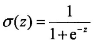
Function image:

From this figure, we can see the following characteristics of sigmoid activation function:
1. When the input is greater than zero, the output must be greater than 0.5
2. When the input exceeds 6, the output will be infinitely close to 1, and the discrimination function of this function will fail
3. The threshold of the function is between 0 and 1
4. Good symmetry
According to the above characteristics, we can preliminarily summarize the application scenarios of sigmoid function: the output of sigmoid is between 0 and 1. In the second classification task, we use the event probability of sigmoid output, that is, when the output meets a certain probability condition, we classify it. Therefore, sigmoid function is suitable as the output layer of second classification problem.
Let's have a deeper understanding of sigmoid function from several angles:
I Explain sigmoid activation function through examples in life:
Title: given the height, weight and daily exercise duration of a sample of experimenters, guess the experimenter's gender.
Firstly, according to the characteristics of sigmoid, that is, when the input is greater than 6, the function will basically fail. Then we set the maximum score for judging height, weight and daily exercise duration as 6. Here, first estimate someone's height as 5, weight as 4.4, waist circumference as 4 and exercise duration as 4.3
Then set the weight of height as 0.3, weight as 4.4, waist circumference as 0.2 and exercise duration as 0.2
For thresholds, set 0 to 0.6 for girls and 0.6 to 1 for boys

Through the above calculation, the result is 0.96, and it is judged that the person is likely to be a boy.
However, after many calculations, the author found that the input value of the method of replacing height and weight by score is still too large. If most of the input numbers are about 3, it is concluded that they are basically above 0.9, which is difficult to have a good discrimination effect. Therefore, in the following, cm is used to calculate height, ton is used to calculate weight, and hour is used to calculate exercise time, Simplify the waistline first and calculate it again.

In the above calculation, the threshold dividing point is changed from 0.5 to 0.62 through the first calculation, so the gender is determined.
It can be seen from the above experiments that sigmoid activation function is suitable for the binary classification experiment in the output layer to output the results.
II Through bp neural network code experiment sigmoid activation function
sigmoid function code definition:
def sigmoid(x):
    return 1 / (1 + np.exp(-x))
The sigmoid activation function is used to realize the complete code of bp neural network. The neural network predicts whether the next high jump will succeed or fail through the previous high jump results, where 1 represents success and 0 represents failure:
import numpy as np
def sigmoid(x):
return 1 / (1 + np.exp(-x))
def main():
# 14 data
data = np.array([
[1, 0, 0, 1, 0, 1, 1, 1],
[0, 0, 1, 1, 0, 0, 1, 0],
[1, 1, 0, 1, 1, 1, 0, 1],
[0, 1, 0, 1, 0, 0, 1, 1],
[1, 0, 1, 1, 0, 1, 1, 1],
[1, 1, 0, 0, 1, 1, 1, 0],
[0, 0, 0, 1, 0, 0, 1, 1],
[1, 0, 1, 1, 0, 1, 1, 1],
[1, 1, 0, 1, 0, 1, 0, 1],
[1, 0, 0, 0, 1, 0, 1, 1],
[1, 0, 0, 1, 0, 1, 1, 0],
[0, 0, 1, 1, 0, 1, 0, 1],
[1, 0, 0, 1, 0, 0, 1, 1],
[0, 1, 0, 1, 0, 1, 1, 1]])
print("raw data:\n", data)
# Article 14 high jump performance of data
highJump = np.array(
[0, 1, 0, 1, 0, 1, 0, 1, 1, 1, 0, 1, 0, 0])
print("Article 14 high jump performance of data:\n", highJump)
# Article 15 data input
data15 = np.array([0, 1, 0, 1, 1, 0, 1, 0])
print("Article 15 data input:\n", data15)
# Set the weight and threshold between the input layer and the hidden layer
wInput = np.random.random(size=(6, 8)) / 10
print("Six sets of weights between input layer and hidden layer:\n", wInput)
bInput = np.random.random(size=(6, 8)) / 10
print("Six sets of thresholds between input layer and hidden layer:\n", bInput)
# Set the weight and threshold between the hidden layer and the output layer
wOutput = np.random.random(size=6) / 10
print("A set of weights between the hidden layer and the output layer", wOutput)
bOutput = np.random.random(size=6) / 10
print("A set of thresholds between the hidden layer and the output layer", bOutput)
loss = 2
count = 0
while loss > 1.7489:
count = count + 1
loss = 0
outputNode = []
for i in range(0, 14):
# Forward propagation
# Calculate hidden layer node input
hide = []
for j in range(0, 6):
hideNode = 0
for k in range(0, 8):
hideNode = data[i, k] * wInput[j, k] + \
bInput[j, k] + hideNode
#print(hideNode)
hideNode = sigmoid(hideNode) # Activation function
hide.append(hideNode)
hide = np.array(hide)
# print("hidden layer node", hide)
output = 0
for j in range(0, 6):
output = hide[j] * wOutput[j] + bOutput[j] + output
output = sigmoid(output)
outputNode.append(output)
# print("output layer node", output)
loss = ((output - highJump[i]) * (output - highJump[i])) / 2 + loss
outputNode = np.array(outputNode)
# Back propagation
# print("hidden layer node", hide)
for i in range(0, 14):
# Update of weight threshold between hidden layer and output layer
wOutputLoss = []
for j in range(0, 6):
wOutputLoss.append((outputNode[i] - highJump[i]) *
outputNode[i] * (1 - outputNode[i])
* hide[j])
wOutputLoss = np.array(wOutputLoss)
# print("wOutputLoss", wOutputLoss)
bOutputLoss = []
for j in range(0, 6):
bOutputLoss.append((outputNode[i] - highJump[i]) *
outputNode[i] * (1 - outputNode[i]))
bOutputLoss = np.array(bOutputLoss)
# print("bOutputLoss", bOutputLoss)
for j in range(0, 6):
wOutput[j] = wOutput[j] - 0.1 * wOutputLoss[j]
bOutput[j] = bOutput[j] - 0.1 * bOutputLoss[j]
# print("updated weight and threshold of hidden layer and output layer", wutput, boutput)
# Weight update between input layer and hidden layer
wInputLoss = np.ones((6, 8)) * 0
for j in range(0, 6):
for k in range(0, 8):
wInputLoss[j][k] = ((outputNode[i] - highJump[i]) *
outputNode[i] *
(1 - outputNode[i]) * wOutput[j]
* hide[j] * (1 - hide[j]) * data[i][k])
wInputLoss = np.array(wInputLoss)
# print("wIutputLoss", wInputLoss)
bInputLoss = np.ones((6, 8)) * 0
for j in range(0, 6):
for k in range(0, 8):
bInputLoss[j][k] = ((outputNode[i] - highJump[i]) *
outputNode[i] * (1 - outputNode[i]) *
wOutput[j] * hide[j] * (1 - hide[j]))
bInputLoss = np.array(bInputLoss)
#print("bIutputLoss", bInputLoss)
for j in range(0, 6):
for k in range(0, 8):
wInput[j][k] = wInput[j][k] - 0.1 * wInputLoss[j][k]
bInput[j][k] = bInput[j][k] - 0.1 * bInputLoss[j][k]
#print("updated weight and threshold between input layer and hidden layer", wunput, binput)
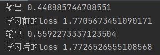
print("output", output)
print("Pre study loss", loss)
loss = 0
for i in range(0, 14):
# Forward propagation
# Calculate hidden layer node input
hide = []
for j in range(0, 6):
hideNode = 0
for k in range(0, 8):
hideNode = data[i, k] * wInput[j, k] + \
bInput[j, k] + hideNode
hideNode = sigmoid(hideNode) # Activation function
hide.append(hideNode)
hide = np.array(hide)
output = 0
for j in range(0, 6):
output = hide[j] * wOutput[j] + bOutput[j] + output
output = sigmoid(output)
loss = ((output - highJump[i]) * (output - highJump[i])) / 2 + loss
print("output", output)
print("After study loss", loss)
# forecast
hide = []
for j in range(0, 6):
hideNode = 0
for k in range(0, 8):
hideNode = data15[k] * wInput[j, k] + \
bInput[j, k] + hideNode
hideNode = sigmoid(hideNode) # Activation function
hide.append(hideNode)
hide = np.array(hide)
output = 0
for j in range(0, 6):
output = hide[j] * wOutput[j] + bOutput[j] + output
output = sigmoid(output)
print(output)
print(loss)
print(count)
if __name__ == '__main__':
main()The bp neural network includes an input layer with eight neurons (that is, eight 01 scores in the original data), a hidden layer with six neurons and an output layer with one neuron.
The results obtained after running the code:
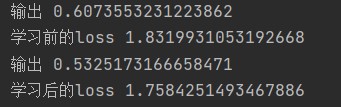
The figure above shows the output and loss of the network before and after learning for the first time
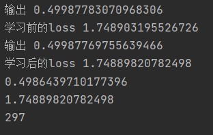
The above figure shows the output and loss before and after the 297th learning, and outputs the final output and loss. It can be seen that the final output is less than 0.5, which predicts that it is more likely to fail in the next test.
- tanh activation function
Function expression:
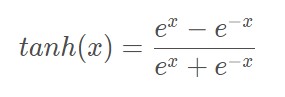
Function image:

Tanh function is also called hyperbolic tangent function, and its value range is [- 1,1]. Tanh function is a deformation of sigmoid, and tanh function is 0-means, so tanh will be better than sigmoid in practical application.
According to the above figure, several features of tanh function can be obtained by combining sigmoid function:
1. Hyperbolic tangent function. The output of tanh function is centered on 0 and the interval is [− 1,1]. Tanh can be imagined as two sigmoid functions together, and the performance is higher than sigmoid function
2. The convergence speed is faster than Sigmoid
3. However, there are still problems of gradient saturation and exp calculation.
According to the above characteristics, we can preliminarily summarize the application scenarios of tanh function: since tanh is an improved version of sigmoid, the application scenarios of sigmoid function tanh can also be used, and the performance of tanh is better. Therefore, when the activation function is uncertain, the priority of using tanh is only after relu, which is different from the characteristics that sigmoid function is applicable to the output layer, The tanh function can also be applied to hidden layers and more.
As before, let's understand the tanh function from two angles
I Explain tanh activation function through examples in life:
Questions before use: know the height, weight and daily exercise duration of a sample of experimenters, and guess the gender of experimenters.

The gender can be determined in the above threshold, and the tanh function can be used in the scene where sigmoid is applicable.
II Through bp neural network code experiment, tanh activation function
tanh function definition code:
def tanh(x):
    return np.sinh(x)/np.cosh(x)
Using the high jump prediction code above, the following code is obtained with slight modification:
import numpy as np


def tanh(x):
    return np.sinh(x)/np.cosh(x)


def main():
    # 14 data
    data = np.array([
        [1, 0, 0, 1, 0, 1, 1, 1],
        [0, 0, 1, 1, 0, 0, 1, 0],
        [1, 1, 0, 1, 1, 1, 0, 1],
        [0, 1, 0, 1, 0, 0, 1, 1],
        [1, 0, 1, 1, 0, 1, 1, 1],
        [1, 1, 0, 0, 1, 1, 1, 0],
        [0, 0, 0, 1, 0, 0, 1, 1],
        [1, 0, 1, 1, 0, 1, 1, 1],
        [1, 1, 0, 1, 0, 1, 0, 1],
        [1, 0, 0, 0, 1, 0, 1, 1],
        [1, 0, 0, 1, 0, 1, 1, 0],
        [0, 0, 1, 1, 0, 1, 0, 1],
        [1, 0, 0, 1, 0, 0, 1, 1],
        [0, 1, 0, 1, 0, 1, 1, 1]])
    print("raw data:\n", data)
    # Article 14 high jump performance of data
    highJump = np.array(
        [0, 1, 0, 1, 0, 1, 0, 1, 1, 1, 0, 1, 0, 0])
    print("Article 14 high jump performance of data:\n", highJump)
    # Article 15 data input
    data15 = np.array([0, 1, 0, 1, 1, 0, 1, 0])
    print("Article 15 data input:\n", data15)
    # Set the weight and threshold between the input layer and the hidden layer
    wInput = np.random.random(size=(6, 8)) / 10
    print("Six sets of weights between input layer and hidden layer:\n", wInput)
    bInput = np.random.random(size=(6, 8)) / 10
    print("Six sets of thresholds between input layer and hidden layer:\n", bInput)
    # Set the weight and threshold between the hidden layer and the output layer
    wOutput = np.random.random(size=6) / 10
    print("A set of weights between the hidden layer and the output layer", wOutput)
    bOutput = np.random.random(size=6) / 10
    print("A set of thresholds between the hidden layer and the output layer", bOutput)
    loss = 2
    count = 0
    while loss < 2.1:
        count = count + 1
        loss = 0
        outputNode = []
        for i in range(0, 14):

            # Forward propagation
            # Calculate hidden layer node input
            hide = []
            for j in range(0, 6):
                hideNode = 0
                for k in range(0, 8):
                    hideNode = data[i, k] * wInput[j, k] + \
                               bInput[j, k] + hideNode
                #print(hideNode)
                hideNode = tanh(hideNode)  # Activation function
                hide.append(hideNode)
            hide = np.array(hide)
            # print("hidden layer node", hide)
            output = 0
            for j in range(0, 6):
                output = hide[j] * wOutput[j] + bOutput[j] + output
            output = tanh(output)
            outputNode.append(output)
            # print("output layer node", output)
            loss = ((output - highJump[i]) * (output - highJump[i])) / 2 + loss
        outputNode = np.array(outputNode)
        # Back propagation
        # Hidden node ("print", hidden layer)
        for i in range(0, 14):
            # Update of weight threshold between hidden layer and output layer
            wOutputLoss = []
            for j in range(0, 6):
                wOutputLoss.append((outputNode[i] - highJump[i]) *
                                   outputNode[i] * (1 - outputNode[i])
                                   * hide[j])
            wOutputLoss = np.array(wOutputLoss)
            # print("wOutputLoss", wOutputLoss)
            bOutputLoss = []
            for j in range(0, 6):
                bOutputLoss.append((outputNode[i] - highJump[i]) *
                                   outputNode[i] * (1 - outputNode[i]))
            bOutputLoss = np.array(bOutputLoss)
            # print("bOutputLoss", bOutputLoss)
            for j in range(0, 6):
                wOutput[j] = wOutput[j] - 0.1 * wOutputLoss[j]
                bOutput[j] = bOutput[j] - 0.1 * bOutputLoss[j]
            # print("updated weight and threshold of hidden layer and output layer", wutput, boutput)
            # Weight update between input layer and hidden layer
            wInputLoss = np.ones((6, 8)) * 0
            for j in range(0, 6):
                for k in range(0, 8):
                    wInputLoss[j][k] = ((outputNode[i] - highJump[i]) *
                                        outputNode[i] *
                                        (1 - outputNode[i]) * wOutput[j]
                                        * hide[j] * (1 - hide[j]) * data[i][k])
            wInputLoss = np.array(wInputLoss)
            # print("wIutputLoss", wInputLoss)
            bInputLoss = np.ones((6, 8)) * 0
            for j in range(0, 6):
                for k in range(0, 8):
                    bInputLoss[j][k] = ((outputNode[i] - highJump[i]) *
                                        outputNode[i] * (1 - outputNode[i]) *
                                        wOutput[j] * hide[j] * (1 - hide[j]))
            bInputLoss = np.array(bInputLoss)
            #print("bIutputLoss", bInputLoss)
            for j in range(0, 6):
                for k in range(0, 8):
                    wInput[j][k] = wInput[j][k] - 0.1 * wInputLoss[j][k]
                    bInput[j][k] = bInput[j][k] - 0.1 * bInputLoss[j][k]
            #print("updated weight and threshold between input layer and hidden layer", wunput, binput)
        print("output", output)
        print("Pre study loss", loss)
        loss = 0
        for i in range(0, 14):
            # Forward propagation
            # Calculate hidden layer node input
            hide = []
            for j in range(0, 6):
                hideNode = 0
                for k in range(0, 8):
                    hideNode = data[i, k] * wInput[j, k] + \
                               bInput[j, k] + hideNode
                hideNode = tanh(hideNode)  # Activation function
                hide.append(hideNode)
            hide = np.array(hide)
            output = 0
            for j in range(0, 6):
                output = hide[j] * wOutput[j] + bOutput[j] + output
            output = tanh(output)
            loss = ((output - highJump[i]) * (output - highJump[i])) / 2 + loss
        print("output", output)
        print("After study loss", loss)

    # forecast
    hide = []
    for j in range(0, 6):
        hideNode = 0
        for k in range(0, 8):
            hideNode = data15[k] * wInput[j, k] + \
                       bInput[j, k] + hideNode
            hideNode = tanh(hideNode)  # Activation function
        hide.append(hideNode)
    hide = np.array(hide)
    output = 0
    for j in range(0, 6):
        output = hide[j] * wOutput[j] + bOutput[j] + output
    output = tanh(output)
    print(output)
    print(loss)
    print(count)


if __name__ == '__main__':
    main()
The above code has the same layers as the previous bp neural network, and each layer has the same neurons. Only the loss result and activation function are modified.
The running results of the above code at the beginning are shown in the figure:
Results the code after multiple learning is shown in the figure:
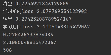
It can be seen that after 506 times of learning, the loss value after learning is larger, which may be caused by problems such as over fitting,
However, it can be preliminarily determined that this code is not very suitable for tanh activation function compared with sigmoid function. It can also be seen that the effect of using tanh for output layer in this code is not as good as sigmoid.
- relu activation function
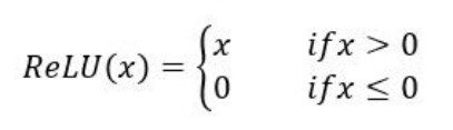
relu function:
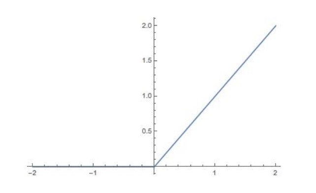
relu function image:
Usage of relu function:
1. In the second classification problem, relu is used except for the output layer
2. relu is generally preferred in case of uncertainty
3. The negative number in relu will directly become 0
4. relu will also be used when encountering dead neurons
Features of relu function:
Rectified linear unit (ReLU) is the most commonly used activation function in modern neural networks. Most feedforward neural networks use the activation function by default.
advantage:
1. The convergence speed of SGD algorithm using ReLU is faster than sigmoid and tanh.
2. In the region of x > 0, there will be no problem of gradient saturation and gradient disappearance.
3. Low computational complexity, no exponential operation is required, and the activation value can be obtained as long as a threshold.
Disadvantages:
The output of ReLU is not the mean value of 0 (subtract the average value of all pixel values on the training set from the value of each pixel. For example, the average value of all pixel points has been calculated to be 128, so after subtracting 128, the current pixel value range is [- 128127], that is, the mean value is zero.) of
I will not calculate the example of relu function again. The basic algorithm idea and code are the same as above.