After sequencing, we can observe the presence of different subtypes of mutations based on the data of different genotypes.

There is only one file to be prepared. The format is as follows:

 

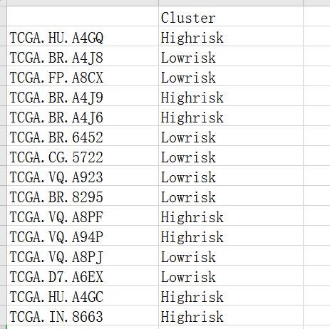
This is the risk model I analyzed in TCGA gastric cancer (STAD) database. The gastric cancer data is divided into high and low risks, and the data can be saved in csv format.

To start running the code, you need to download the TCGAbiolinks software package. Based on this R package, you can use the R software to download any data in TCGA. The only disadvantage is that it runs slowly. Let's download the STAD mutation data in TCGA:

rm(list = ls())
BiocManager::install("TCGAbiolinks",ask = F,update = F)
library(TCGAbiolinks)
library(maftools)

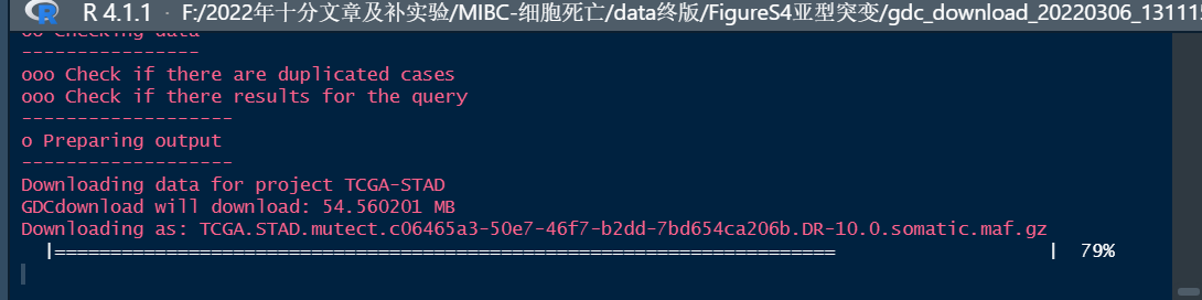
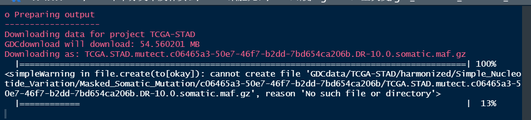
mut <- GDCquery_Maf(tumor = "STAD",pipelines = "mutect2") #Download mutation data
dim(mut)

Because TCGA has different abbreviations of different cancers, for example, bladder cancer is BLCA and lung adenocarcinoma is LUAD. Therefore, if we want to download the mutation data of any cancer, we suggest using TCGA official abbreviation. The download progress will be displayed after running here. You need to wait for dozens of minutes here.

 

 

After downloading, you can check the sample name in the STAD mutation data:

mut$Tumor_Sample_Barcode[1]## View sample name

 

It can be seen that the sample name of STAD mutation data is different from that of my risk subtype data, so it needs to be changed to the same name. We can use substr and gsub to shorten and replace the name:

mut$Tumor_Sample_Barcode <- substr(mut$Tumor_Sample_Barcode,1,12)
mut$Tumor_Sample_Barcode <- gsub("-",".",mut$Tumor_Sample_Barcode)

Then download the subtype file:

rt <- read.csv("BLCA_cluster.csv",header = T,sep = ",")
head(rt)

The mutation data of high-risk and low-risk subtypes are extracted based on the subtype file:

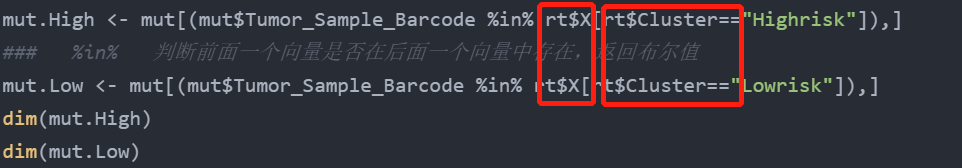
mut.High <- mut[(mut$Tumor_Sample_Barcode %in% rt$X[rt$Cluster=="Highrisk"]),]
###   %In% determines whether the previous vector exists in the next vector and returns a Boolean value
mut.Low <- mut[(mut$Tumor_Sample_Barcode %in% rt$X[rt$Cluster=="Lowrisk"]),]
dim(mut.High)
dim(mut.Low)

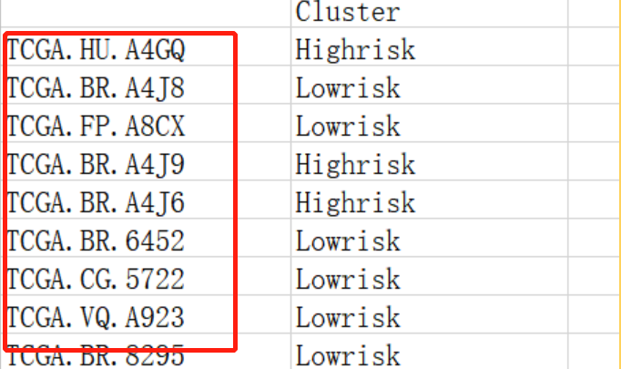
Note the selection of column names after the dollar sign here. The first red box selects the first column of subtype file, and the second red box selects the second column of subtype file:

Let's start the waterfall diagram, download the maftools package, load the maftools package and read the data:

library(maftools)
maf.High <- read.maf(maf=mut.High,isTCGA=T)## Reading mutation data for high-risk subtypes
maf.Low <- read.maf(maf = mut.Low,isTCGA = T)## Reading mutation data for low-risk subtypes
maf.all <- read.maf(maf = mut,isTCGA = T)## Read the total sample mutation data

Set the color, race and other information below. The code here does not need to be modified:

col = RColorBrewer::brewer.pal(n = 10, name = 'Paired')
names(col) = c('Frame_Shift_Del','Missense_Mutation', 'Nonsense_Mutation', 'Frame_Shift_Ins','In_Frame_Ins', 'Splice_Site', 'In_Frame_Del','Nonstop_Mutation','Translation_Start_Site','Multi_Hit')

#race
racecolors = RColorBrewer::brewer.pal(n = 4,name = 'Spectral')
names(racecolors) = c("ASIAN", "WHITE", "BLACK_OR_AFRICAN_AMERICAN",  "AMERICAN_INDIAN_OR_ALASKA_NATIVE")

Now start to draw the general waterfall diagram. The code and picture are as follows:

oncoplot(maf = maf.all,
         colors = col,#Color mutation
         top = 20)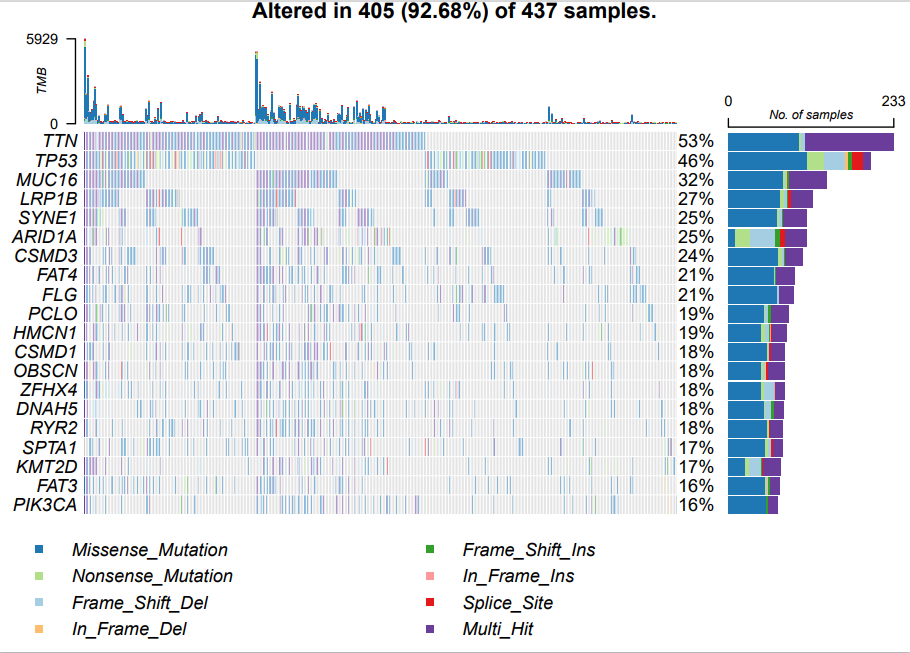

Draw the waterfall map of high-risk subtypes. The codes and pictures are as follows:

oncoplot(maf = maf.high,
         colors = col,#Color mutation
         top = 20)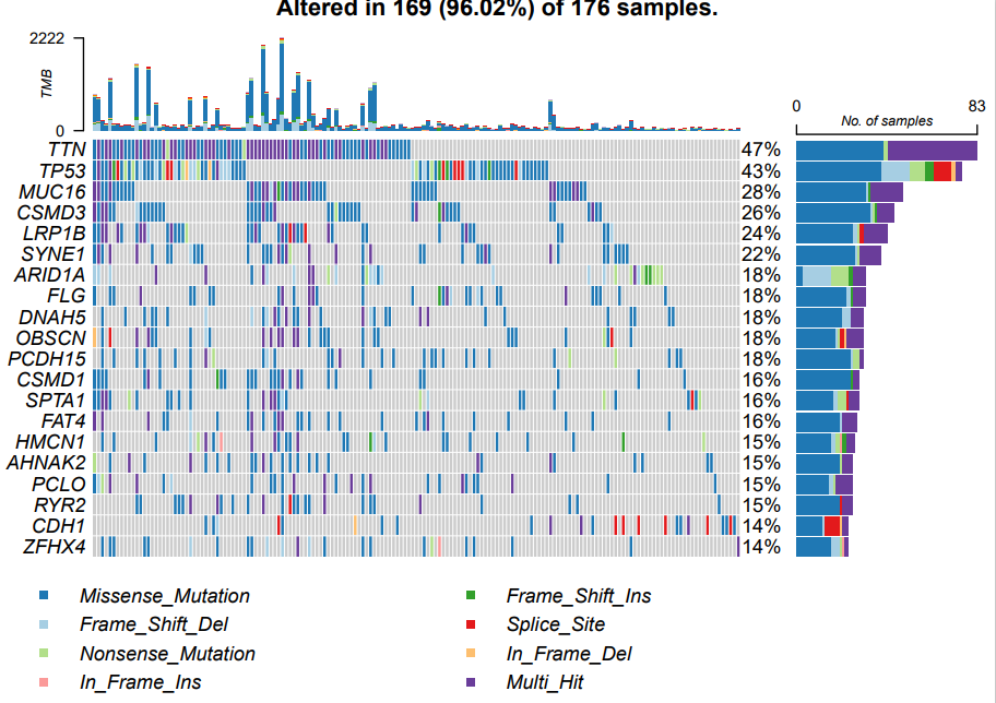

Draw a low-risk waterfall diagram. The code and picture are as follows:

oncoplot(maf = maf.low,
         colors = col,#Color mutation
         top = 20)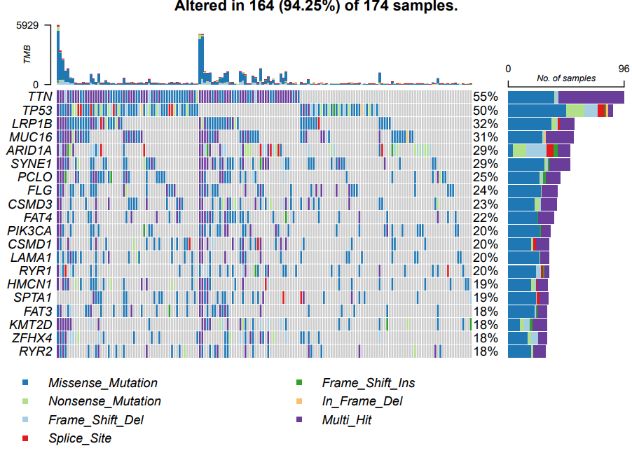

 

If the prognosis of patients with different subtypes is different, the genes with the highest mutation rate and mutation load will also be different. As shown in the above figure, except for TNN and TP53, the later gene ranking and mutation rate are significantly different.