MySQL notes: Chapter 08_ Aggregate function

Posted by rcarr on Sat, 05 Mar 2022 15:50:16 +0100

Note: this content is compiled from the MySQL video of Shangshan Silicon Valley Station B >>MySQL video of Shangsi valley station B
The previous chapter talked about SQL single line functions. In fact, there is another kind of SQL function, which is called aggregation (or aggregation, grouping) function. It is a function that summarizes a group of data. The input is a collection of a group of data and the output is a single value.

1. Introduction to aggregate function

What is an aggregate function
The aggregate function acts on a set of data and returns a value to a set of data.

Aggregate function type
AVG()
SUM()
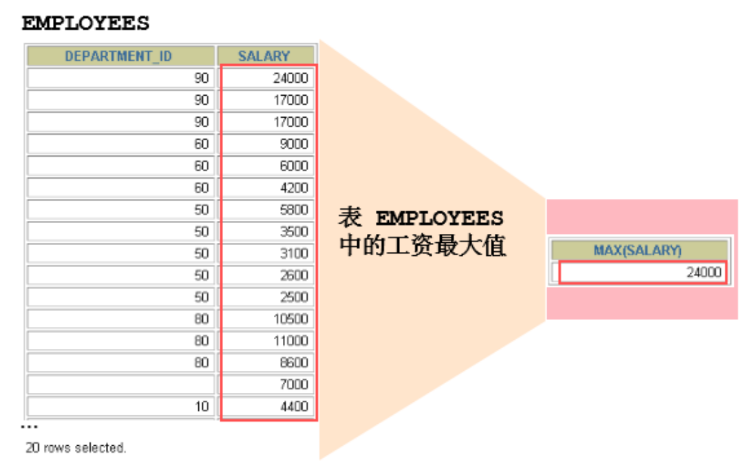
MAX()
MIN()
COUNT()

Aggregate function syntax

1.1 AVG and SUM functions

AVG and SUM functions can be used for numerical data.

 SELECT AVG(salary), MAX(salary),MIN(salary), SUM(salary) FROM employees WHERE job_id LIKE '%REP%';
/*
+-------------+-------------+-------------+-------------+
| AVG(salary) | MAX(salary) | MIN(salary) | SUM(salary) |
+-------------+-------------+-------------+-------------+
| 8272.727273 |    11500.00 |     6000.00 |   273000.00 |
+-------------+-------------+-------------+-------------+
*/

1.2 MIN and MAX functions

You can use the MIN and MAX functions for any data type.

SELECT MIN(hire_date), MAX(hire_date)
FROM employees;
/*
+----------------+----------------+
| MIN(hire_date) | MAX(hire_date) |
+----------------+----------------+
| 1987-06-17     | 2000-04-21     |
+----------------+----------------+
*/

1.3 COUNT function

COUNT(*) returns the total number of records in the table, applicable to any data type.

SELECT COUNT(*)
FROM employees
WHERE department_id = 50;
/*
+----------+
| COUNT(*) |
+----------+
|       45 |
+----------+
*/

COUNT(expr) returns the total number of records whose expr is not empty.

SELECT COUNT(commission_pct)
FROM employees
WHERE department_id = 50;
/*
+-----------------------+
| COUNT(commission_pct) |
+-----------------------+
|                     0 |
+-----------------------+
*/

Question: who can use count(*), count(1), count (column name)?
In fact, there is no difference for the tables of MyISAM engine. There is a counter inside this engine to maintain the number of rows.

The table of InnoDB engine uses count(*) and count(1) to directly read the number of rows. The complexity is O(n), because InnoDB really needs to count it again. But better than the specific count (column name).

Question: can you replace count(*) with count (column name)?
Do not use count (column name) instead of count(*). count(*) is the syntax of standard statistics rows defined by SQL92. It has nothing to do with the database, NULL and non NULL.
Note: count(*) will count the rows with NULL value, while count (column name) will not count the rows with NULL value.

Demo code

#1. Several common aggregate functions
#1.1 AVG / SUM: only applicable to fields (or variables) of numerical type

SELECT AVG(salary),SUM(salary),AVG(salary) * 107
FROM employees;
/*output
+-------------+-------------+-------------------+
| AVG(salary) | SUM(salary) | AVG(salary) * 107 |
+-------------+-------------+-------------------+
| 6461.682243 |   691400.00 |     691400.000000 |
+-------------+-------------+-------------------+
*/
#The following actions are meaningless
SELECT SUM(last_name),AVG(last_name),SUM(hire_date)
FROM employees;


#1.2 MAX / MIN: applicable to fields (or variables) of numeric type, string type and date time type
SELECT MAX(salary),MIN(salary)
FROM employees;
/*output
+-------------+-------------+
| MAX(salary) | MIN(salary) |
+-------------+-------------+
|    24000.00 |     2100.00 |
+-------------+-------------+
*/
SELECT MAX(last_name),MIN(last_name),MAX(hire_date),MIN(hire_date)
FROM employees;
/*output
+----------------+----------------+----------------+----------------+
| MAX(last_name) | MIN(last_name) | MAX(hire_date) | MIN(hire_date) |
+----------------+----------------+----------------+----------------+
| Zlotkey        | Abel           | 2000-04-21     | 1987-06-17     |
+----------------+----------------+----------------+----------------+
*/

#1.3 COUNT: 
# ① Function: calculate the number of specified fields in the query structure (excluding NULL values)
SELECT COUNT(employee_id),COUNT(salary),COUNT(2 * salary),COUNT(1),COUNT(2),COUNT(*)
FROM employees ;
/*Output:
+--------------------+---------------+-------------------+----------+----------+----------+
| COUNT(employee_id) | COUNT(salary) | COUNT(2 * salary) | COUNT(1) | COUNT(2) | COUNT(*) |
+--------------------+---------------+-------------------+----------+----------+----------+
|                107 |           107 |               107 |      107 |      107 |      107 |
+--------------------+---------------+-------------------+----------+----------+----------+
*/

SELECT *
FROM employees;

#How many records are there in the calculation table?
#Method 1: COUNT(*)
#Mode 2: COUNT(1)
#Method 3: count (specific field): not necessarily true!

#② Note: when calculating the number of occurrences of the specified field, the NULL value is not calculated.
SELECT COUNT(commission_pct)#Count (specific field)
FROM employees;
/*
+-----------------------+
| COUNT(commission_pct) |
+-----------------------+
|                    35 |
+-----------------------+
*/
SELECT commission_pct#Specific field
FROM employees
WHERE commission_pct IS NOT NULL;
/* 35 Records
+----------------+
| commission_pct |
+----------------+
|           0.40 |
|           0.30 |
|           0.30 |
*/

#③ Formula: AVG = SUM / COUNT (it is true whether there is a null value or not)
SELECT AVG(salary),SUM(salary)/COUNT(salary),
AVG(commission_pct),SUM(commission_pct)/COUNT(commission_pct),
SUM(commission_pct) / 107
FROM employees;
/*
+-------------+---------------------------+---------------------+-------------------------------------------+---------------------------+
| AVG(salary) | SUM(salary)/COUNT(salary) | AVG(commission_pct) | SUM(commission_pct)/COUNT(commission_pct) | SUM(commission_pct) / 107 |
+-------------+---------------------------+---------------------+-------------------------------------------+---------------------------+
| 6461.682243 |               6461.682243 |            0.222857 |                                  0.222857 |                  0.072897 |
+-------------+---------------------------+---------------------+-------------------------------------------+---------------------------+
*/

#Demand: query the average bonus rate in the company
#FALSE!
SELECT AVG(commission_pct)
FROM employees;

#SUM also does not consider NULL values
#correct:
SELECT SUM(commission_pct) / COUNT(IFNULL(commission_pct,0)),#Equivalent to COUNT(IFNULL(commission_pct,1/2/3/4 /))
AVG(IFNULL(commission_pct,0))
FROM employees;
/*Output:
+-------------------------------------------------------+-------------------------------+
| SUM(commission_pct) / COUNT(IFNULL(commission_pct,0)) | AVG(IFNULL(commission_pct,0)) |
+-------------------------------------------------------+-------------------------------+
|                                              0.072897 |                      0.072897 |
+-------------------------------------------------------+-------------------------------+
*/

# How to count the number of records in the table? Which of COUNT(*), COUNT(1) \ count (constant) and count (specific field) is more efficient?
# If the MyISAM storage engine is used, the efficiency of the three is the same, and the time complexity is O(1)
# If the InnoDB storage engine is used, the efficiency of the three is: count (*) = count (1) > count (field)

2. GROUP BY

2.1 basic use

You can use the GROUP BY clause to divide the data in a table into groups

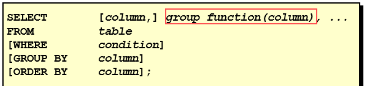
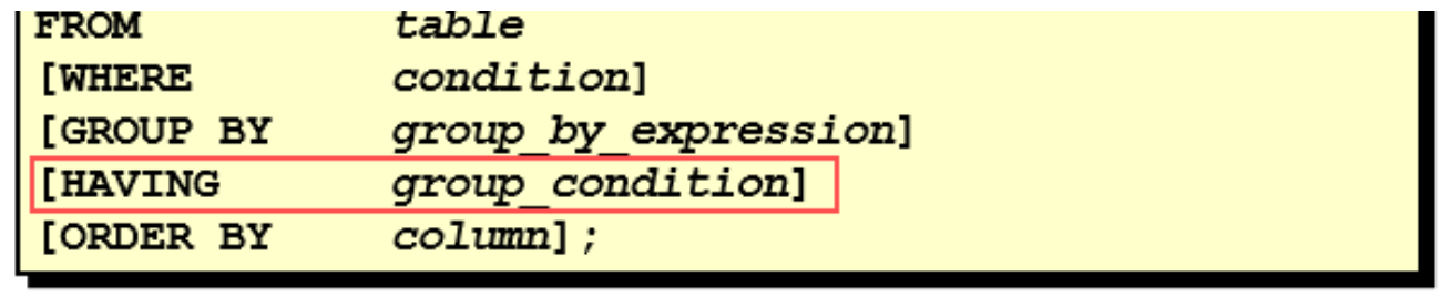
SELECT column, group_function(column)
FROM table
[WHERE condition]
[GROUP BY group_by_expression]
[ORDER BY column];

Clear: WHERE must be placed after FROM

In the SELECT list, all columns not included in the group function should be included in the GROUP BY clause

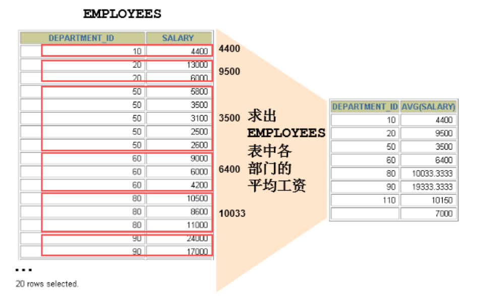
SELECT department_id, AVG(salary)
FROM employees
GROUP BY department_id ;
/*
+---------------+--------------+
| department_id | AVG(salary)  |
+---------------+--------------+
|          NULL |  7000.000000 |
|            10 |  4400.000000 |
|            20 |  9500.000000 |
|            30 |  4150.000000 |
|            40 |  6500.000000 |
|            50 |  3475.555556 |
|            60 |  5760.000000 |
|            70 | 10000.000000 |
|            80 |  8955.882353 |
|            90 | 19333.333333 |
|           100 |  8600.000000 |
|           110 | 10150.000000 |
+---------------+--------------+
*/

Columns included in the GROUP BY clause do not have to be included in the SELECT list

SELECT AVG(salary) FROM employees 
GROUP BY department_id ;
/*
+--------------+
| AVG(salary)  |
+--------------+
|  7000.000000 |
|  4400.000000 |
|  9500.000000 |
|  4150.000000 |
|  6500.000000 |
|  3475.555556 |
|  5760.000000 |
| 10000.000000 |
|  8955.882353 |
| 19333.333333 |
|  8600.000000 |
| 10150.000000 |
+--------------+
*/

2.2 grouping using multiple columns

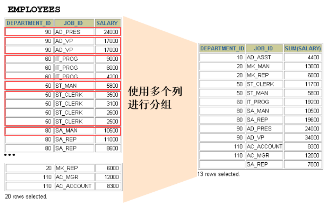
SELECT department_id dept_id, job_id, SUM(salary)
FROM employees
GROUP BY department_id, job_id ;
/*
+---------+------------+-------------+
| dept_id | job_id     | SUM(salary) |
+---------+------------+-------------+
|    NULL | SA_REP     |     7000.00 |
|      10 | AD_ASST    |     4400.00 |
|      20 | MK_MAN     |    13000.00 |
|      20 | MK_REP     |     6000.00 |
|      30 | PU_CLERK   |    13900.00 |
|      30 | PU_MAN     |    11000.00 |
|      40 | HR_REP     |     6500.00 |
|      50 | SH_CLERK   |    64300.00 |
|      50 | ST_CLERK   |    55700.00 |
|      50 | ST_MAN     |    36400.00 |
|      60 | IT_PROG    |    28800.00 |
|      70 | PR_REP     |    10000.00 |
|      80 | SA_MAN     |    61000.00 |
|      80 | SA_REP     |   243500.00 |
|      90 | AD_PRES    |    24000.00 |
|      90 | AD_VP      |    34000.00 |
|     100 | FI_ACCOUNT |    39600.00 |
|     100 | FI_MGR     |    12000.00 |
|     110 | AC_ACCOUNT |     8300.00 |
|     110 | AC_MGR     |    12000.00 |
+---------+------------+-------------+
*/

After using the WITH ROLLUP keyword, add a record after all the queried grouping records. The record calculates the sum of all the queried records, that is, the number of statistical records.

SELECT department_id,AVG(salary)
FROM employees
WHERE department_id > 80
GROUP BY department_id WITH ROLLUP;
/*
+---------------+--------------+
| department_id | AVG(salary)  |
+---------------+--------------+
|            90 | 19333.333333 |
|           100 |  8600.000000 |
|           110 | 10150.000000 |
|          NULL | 11809.090909 |
+---------------+--------------+
*/

be careful:
When using ROLLUP, you cannot use the ORDER BY clause to sort the results at the same time, that is, ROLLUP and ORDER BY are mutually exclusive.

Demo code

#Others: variance, standard deviation, median
#2. Use of group by

#Demand: query the average wage and maximum wage of each department
SELECT department_id,AVG(salary),SUM(salary)
FROM employees
GROUP BY department_id
/*Output:
+---------------+--------------+-------------+
| department_id | AVG(salary)  | SUM(salary) |
+---------------+--------------+-------------+
|          NULL |  7000.000000 |     7000.00 |
|            10 |  4400.000000 |     4400.00 |
|            20 |  9500.000000 |    19000.00 |
|            30 |  4150.000000 |    24900.00 |
|            40 |  6500.000000 |     6500.00 |
|            50 |  3475.555556 |   156400.00 |
|            60 |  5760.000000 |    28800.00 |
|            70 | 10000.000000 |    10000.00 |
|            80 |  8955.882353 |   304500.00 |
|            90 | 19333.333333 |    58000.00 |
|           100 |  8600.000000 |    51600.00 |
|           110 | 10150.000000 |    20300.00 |
+---------------+--------------+-------------+
*/

#Requirement: query each job_ Average salary of ID
SELECT job_id,AVG(salary)
FROM employees
GROUP BY job_id;
/*output
+------------+--------------+
| job_id     | AVG(salary)  |
+------------+--------------+
| AC_ACCOUNT |  8300.000000 |
| AC_MGR     | 12000.000000 |
| AD_ASST    |  4400.000000 |
| AD_PRES    | 24000.000000 |
| AD_VP      | 17000.000000 |
| FI_ACCOUNT |  7920.000000 |
| FI_MGR     | 12000.000000 |
| HR_REP     |  6500.000000 |
| IT_PROG    |  5760.000000 |
| MK_MAN     | 13000.000000 |
| MK_REP     |  6000.000000 |
| PR_REP     | 10000.000000 |
| PU_CLERK   |  2780.000000 |
| PU_MAN     | 11000.000000 |
| SA_MAN     | 12200.000000 |
| SA_REP     |  8350.000000 |
| SH_CLERK   |  3215.000000 |
| ST_CLERK   |  2785.000000 |
| ST_MAN     |  7280.000000 |
+------------+--------------+
*/

#Demand: query each department_ id,job_ Average salary of ID
#Mode 1:
SELECT department_id,job_id,AVG(salary)
FROM employees
GROUP BY  department_id,job_id;
/*Partial output
+---------------+------------+--------------+
| department_id | job_id     | AVG(salary)  |
+---------------+------------+--------------+
|          NULL | SA_REP     |  7000.000000 |
|            10 | AD_ASST    |  4400.000000 |
|            20 | MK_MAN     | 13000.000000 |
|            20 | MK_REP     |  6000.000000 |
|            30 | PU_CLERK   |  2780.000000 |
|            30 | PU_MAN     | 11000.000000 |
|            40 | HR_REP     |  6500.000000 |
|            50 | SH_CLERK   |  3215.000000 |
*/
#Mode 2: mode 1 and mode 2 are actually the same (both grouped by job_id and department_id)
SELECT job_id,department_id,AVG(salary)
FROM employees
GROUP BY job_id,department_id;
/*Partial output
+------------+---------------+--------------+
| job_id     | department_id | AVG(salary)  |
+------------+---------------+--------------+
| AC_ACCOUNT |           110 |  8300.000000 |
| AC_MGR     |           110 | 12000.000000 |
| AD_ASST    |            10 |  4400.000000 |
| AD_PRES    |            90 | 24000.000000 |
| AD_VP      |            90 | 17000.000000 |
| FI_ACCOUNT |           100 |  7920.000000 |
| FI_MGR     |           100 | 12000.000000 |
*/


#Wrong! -- > Select job_ The ID field does not appear in GROUP BY, so there is an error
#The salary in AVG(salary) appears in the group function without error
SELECT department_id,job_id,AVG(salary)
FROM employees
GROUP BY department_id;#Press department only_ Error in ID group Oracle
#The conclusion drawn from the above error:
#Conclusion 1: the fields of non group functions in SELECT must be declared in GROUP BY.
#      Conversely, the fields declared in GROUP BY may not appear in SELECT.
#Conclusion 2: the GROUP BY statement follows FROM, WHERE, ORDER BY and LIMIT
#Conclusion 3: WITH ROLLUP can be used in GROUP BY in MySQL

#Witherup example:
#WITH ROLLUP: after grouping, add the overall group function result at the end
#As in the following example, add AVG(salary) 6461.682243 of all employees at the end 
SELECT department_id,AVG(salary)
FROM employees
GROUP BY department_id WITH ROLLUP;
/*
+---------------+--------------+
| department_id | AVG(salary)  |
+---------------+--------------+
|          NULL |  7000.000000 |
|            10 |  4400.000000 |
|            20 |  9500.000000 |
|            30 |  4150.000000 |
|            40 |  6500.000000 |
|            50 |  3475.555556 |
|            60 |  5760.000000 |
|            70 | 10000.000000 |
|            80 |  8955.882353 |
|            90 | 19333.333333 |
|           100 |  8600.000000 |
|           110 | 10150.000000 |
|          NULL |  6461.682243 |
+---------------+--------------+
*/

#Demand A: query the average salary of each department and arrange it in ascending order
SELECT department_id,AVG(salary) avg_sal
FROM employees
GROUP BY department_id
ORDER BY avg_sal ASC;
/*
+---------------+--------------+
| department_id | avg_sal      |
+---------------+--------------+
|            50 |  3475.555556 |
|            30 |  4150.000000 |
|            10 |  4400.000000 |
|            60 |  5760.000000 |
|            40 |  6500.000000 |
|          NULL |  7000.000000 |
|           100 |  8600.000000 |
|            80 |  8955.882353 |
|            20 |  9500.000000 |
|            70 | 10000.000000 |
|           110 | 10150.000000 |
|            90 | 19333.333333 |
+---------------+--------------+
*/

#Then, requirement A leads to the following description:
#Note: when using ROLLUP, you cannot use the ORDER BY clause to sort the results at the same time, that is, ROLLUP and ORDER BY are mutually exclusive.
#FALSE:
SELECT department_id,AVG(salary) avg_sal
FROM employees
GROUP BY department_id WITH ROLLUP
ORDER BY avg_sal ASC;

3. HAVING

3.1 basic use

Filter grouping: HAVING clause

Rows have been grouped.
Aggregate function used.
Groups that meet the conditions in the HAVING clause are displayed.
HAVING cannot be used alone. It must be used together with GROUP BY.

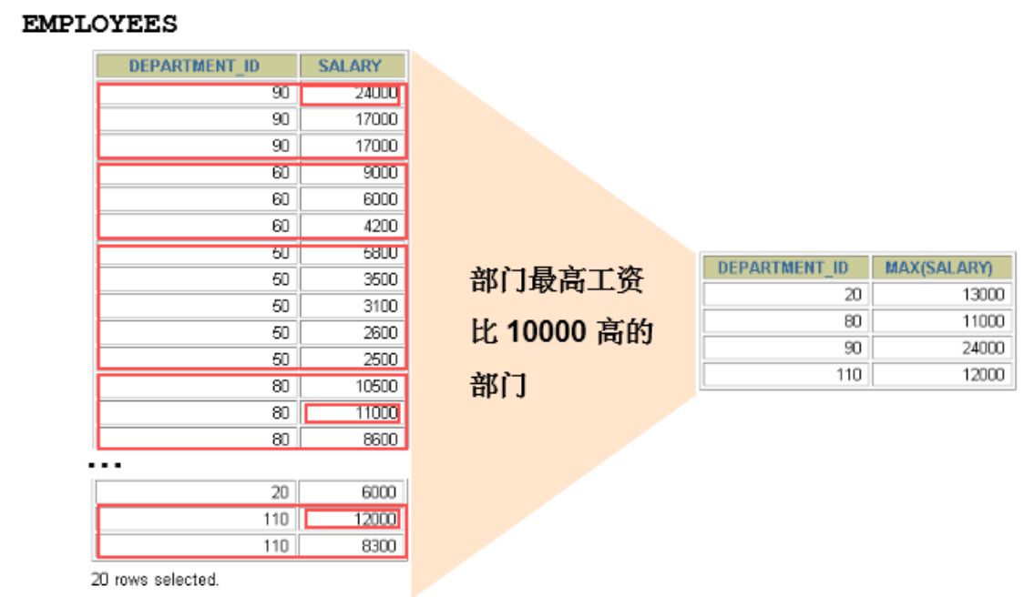
SELECT department_id, MAX(salary)
FROM employees
GROUP BY department_id
HAVING MAX(salary)>10000 ;
/*
+---------------+-------------+
| department_id | MAX(salary) |
+---------------+-------------+
|            20 |    13000.00 |
|            30 |    11000.00 |
|            80 |    14000.00 |
|            90 |    24000.00 |
|           100 |    12000.00 |
|           110 |    12000.00 |
+---------------+-------------+
*/

Illegal use of aggregate function: aggregate function cannot be used in WHERE clause. As follows:

SELECT department_id, AVG(salary)
FROM employees
WHERE AVG(salary) > 8000
GROUP BY department_id;
#report errors:
#ERROR 1111 (HY000): Invalid use of group function

3.2 comparison between where and HAVING

Difference 1: WHERE can directly use the fields in the table as the filter criteria, but cannot use the calculation function in the grouping as the filter criteria; HAVING must be used together with GROUP BY. You can use grouping calculation functions and grouping fields as filtering conditions.

This determines that when grouping statistics is needed, HAVING can complete tasks that WHERE cannot. This is because in the query syntax structure, WHERE is before GROUP BY, so the grouping results cannot be filtered. After HAVING GROUP BY, you can use the grouping field and the calculation function in the grouping to filter the grouping result set. This function cannot be completed by WHERE. In addition, the records excluded by WHERE are no longer included in the group.

Difference 2: if you need to obtain the required data from the association table through connection, WHERE is to filter before connection, while HAVING is to connect first
Post filter.

This determines that WHERE is more efficient than HAVING in association query. Because WHERE can be filtered first and connected with a smaller filtered dataset and associated table, it takes less resources and has high execution efficiency. HAVING needs to prepare the result set first, that is, associate with the unfiltered data set, and then filter this large data set, which takes up more resources and has low execution efficiency.

The summary is as follows:

.	advantage	shortcoming
WHERE	Filter the data first and then associate it, which has high execution efficiency	You cannot filter using a calculated function in a group
HAVING	You can use the calculation function in the group	It is inefficient to filter in the final result set

Selection in development:
WHERE and HAVING are not mutually exclusive. You can use WHERE and HAVING in a query at the same time. Have is used for conditions containing grouping statistical functions, and WHERE is used for general conditions. This not only makes use of the efficiency and speed of WHERE conditions, but also gives play to the advantage that HAVING can use query conditions including grouping statistical functions. When the amount of data is particularly large, the operation efficiency will be very different.

Demo code

#3. Use of having (function: used to filter data) WHERE is also used for filtering
#Exercise: query the information of departments with the highest salary higher than 10000 in each department
#Incorrect wording:
SELECT department_id,MAX(salary)
FROM employees
WHERE MAX(salary) > 10000#WHERE statement after FROM
GROUP BY department_id;


#Requirement 1: if the aggregate function is used in the filter condition, you must use HAVING to replace WHERE. Otherwise, an error is reported.
#Requirement 2: HAVING must be declared after GROUP BY.
#Correct writing:
SELECT department_id,MAX(salary)
FROM employees
GROUP BY department_id
HAVING MAX(salary) > 10000;
#Requirement 3: in development, we use HAVING on the premise that GROUP BY is used in SQL.




#Exercise: query the Department information with the highest salary higher than 10000 in the four departments with department IDs of 10, 20, 30 and 40
#Mode 1: recommended, the execution efficiency is higher than mode 2
SELECT department_id,MAX(salary)
FROM employees
WHERE department_id IN (10,20,30,40)
GROUP BY department_id
HAVING MAX(salary) > 10000;
/*
+---------------+-------------+
| department_id | MAX(salary) |
+---------------+-------------+
|            20 |    13000.00 |
|            30 |    11000.00 |
+---------------+-------------+
*/
#Mode 2:
SELECT department_id,MAX(salary)
FROM employees
GROUP BY department_id
HAVING MAX(salary) > 10000 AND department_id IN (10,20,30,40);
#Conclusion: when there is an aggregate function in the filter condition, the filter condition must be declared in HAVING.
#      When there is no aggregate function in the filter condition, the filter condition can be declared in WHERE or HAVING. However, it is recommended that you declare it in WHERE.

/*
  WHERE Comparison with HAVING
1. In terms of scope of application, HAVING has a wider scope of application. 
2. If there is no aggregation function in the filter condition: in this case, the execution efficiency of WHERE is higher than that of HAVING
*/

4. SELECT execution process

4.1 query structure

#Mode 1:
SELECT ...,....,...
FROM ...,...,....
WHERE Connection conditions of multiple tables
AND Filter conditions without group functions
GROUP BY ...,...
HAVING Filter conditions containing group functions
ORDER BY ... ASC/DESC
LIMIT ...,...
#Mode 2:
SELECT ...,....,...
FROM ... JOIN ...
ON Connection conditions of multiple tables
JOIN ...
ON ...
WHERE Filter group does not contain filter conditions
AND/OR Filter conditions without group functions
GROUP BY ...,...
HAVING Filter conditions containing group functions
ORDER BY ... ASC/DESC
LIMIT ...,...
#Of which:
#(1) From: which tables to filter from
#(2) on: Descartes product is removed when associating multi table queries
#(3) where: criteria to filter from the table
#(4) group by: grouping basis
#(5) having: filter again in the statistical results
#(6) order by: sort
#(7) limit: paging

4.2 SELECT execution sequence

You need to remember the two orders of SELECT query:

The order of keywords cannot be reversed:

SELECT ... FROM ... WHERE ... GROUP BY ... HAVING ... ORDER BY ... LIMIT...

Execution order of SELECT statement (in MySQL and Oracle, the execution order of SELECT is basically the same):

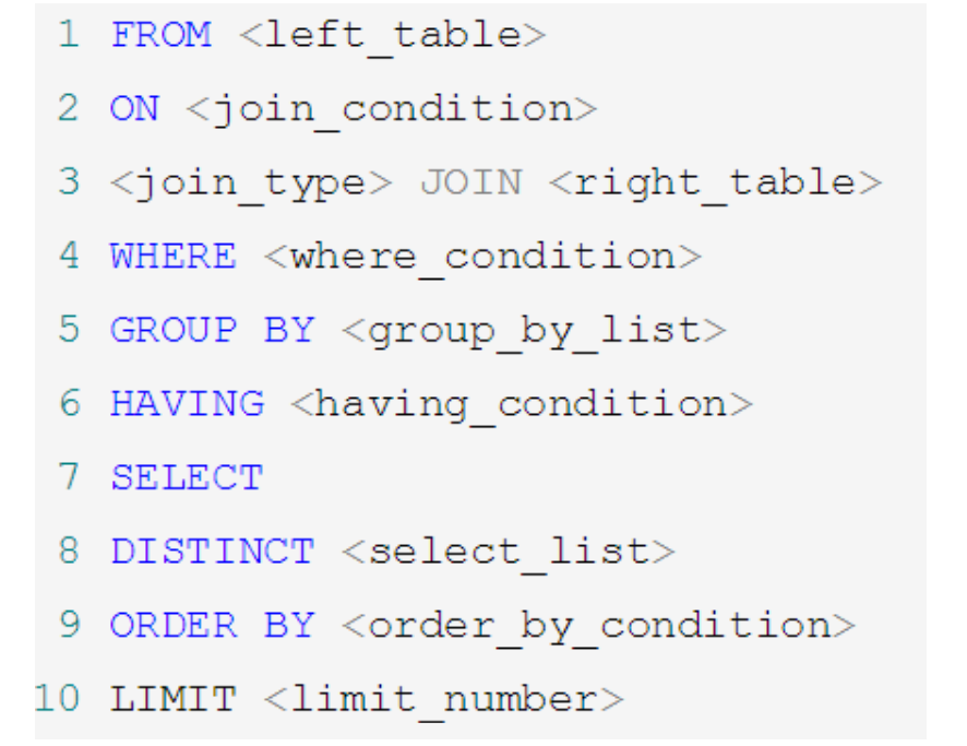
FROM -> WHERE -> GROUP BY -> HAVING -> SELECT Field of -> DISTINCT -> ORDER BY -> LIMIT

For example, if you write an SQL statement, its keyword order and execution order are as follows:

SELECT DISTINCT player_id, player_name, count(*) as num # Sequence 5
FROM player JOIN team ON player.team_id = team.team_id # Sequence 1
WHERE height > 1.80 # Sequence 2
GROUP BY player.team_id # Sequence 3
HAVING num > 2 # Sequence 4
ORDER BY num DESC # Sequence 6
LIMIT 2 # Sequence 7

When the SELECT statement executes these steps, each step will generate a virtual table, and then pass this virtual table into the next step as input. It should be noted that these steps are implicit in the execution of SQL and are invisible to us.

4.3 execution principle of SQL

SELECT executes the FROM step first. At this stage, if you want to perform an associated query on multiple tables, you will go through the following steps:

First, find the Cartesian product through CROSS JOIN, which is equivalent to getting the virtual table vt (virtual table) 1-1;
Filter through ON, filter ON the basis of virtual table vt1-1, and get virtual table vt1-2;
Add an external row. If we use left join, right link or full join, external rows will be involved, that is, add external rows on the basis of virtual table vt1-2 to get virtual table vt1-3.

Of course, if we operate on more than two tables, we will repeat the above steps until all tables are processed. This process yields our raw data.

When we get the original data of the query data table, that is, the final virtual table vt1, we can proceed to the WHERE stage on this basis. In this stage, the virtual table vt2 will be obtained by filtering according to the results of vt1 table.

Then enter the third and fourth steps, that is, the GROUP and HAVING stages. In this stage, the virtual tables vt3 and vt4 are obtained by grouping and grouping filtering based on the virtual table vt2.

After we complete the condition filtering part, we can filter the fields extracted from the table, that is, enter the SELECT and DISTINCT stages.

First, the desired fields will be extracted in the SELECT phase, and then the duplicate rows will be filtered out in the DISTINCT phase to obtain the intermediate virtual tables respectively
vt5-1 and vt5-2.

After we extract the desired field data, we can sort according to the specified field, that is, the ORDER BY stage to get the virtual table vt6.

Finally, on the basis of vt6, take out the records of the specified row, that is, the LIMIT stage, and get the final result, which corresponds to the virtual table vt7.

Of course, when writing a SELECT statement, there may not be all keywords, and the corresponding stage will be omitted. At the same time, because SQL is a structured query language similar to English, we should also pay attention to the corresponding keyword order when writing the SELECT statement. The so-called underlying operation principle is the execution order we just talked about.

Demo code

#4. SQL underlying execution principle
#4.1 complete structure of select statement
/*
#sql92 Syntax:
SELECT ....,....,....((aggregate function exists)
FROM ...,....,....
WHERE The join condition AND of multiple tables does not contain the filter condition of aggregate function
GROUP BY ...,....
HAVING Filter conditions containing aggregate functions
ORDER BY ....,...(ASC / DESC )
LIMIT ...,....


#sql99 Syntax:
SELECT ....,....,....((aggregate function exists)
FROM ... (LEFT / RIGHT)JOIN ....ON Connection conditions of multiple tables 
(LEFT / RIGHT)JOIN ... ON ....
WHERE Filter condition without aggregate function
GROUP BY ...,....
HAVING Filter conditions containing aggregate functions
ORDER BY ....,...(ASC / DESC )
LIMIT ...,....
*/

#4.2 execution process of SQL statement:
#FROM ...,...-> ON -> (LEFT/RIGNT  JOIN) -> WHERE -> GROUP BY -> HAVING -> SELECT -> DISTINCT -> 
# ORDER BY -> LIMIT

After class practice

# Chapter 08_ After class exercise of aggregate function
#1. Can the where clause use group functions for filtering? No!

#2. Query the maximum value, minimum value, average value and total of employee salary of the company
SELECT MAX(salary) max_sal ,MIN(salary) mim_sal,AVG(salary) avg_sal,SUM(salary) sum_sal
FROM employees;
/*output
+----------+---------+-------------+-----------+
| max_sal  | mim_sal | avg_sal     | sum_sal   |
+----------+---------+-------------+-----------+
| 24000.00 | 2100.00 | 6461.682243 | 691400.00 |
+----------+---------+-------------+-----------+
*/

#3. Query each job_ The maximum value, minimum value, average value and sum of employee salary of ID
SELECT job_id,MAX(salary),MIN(salary),AVG(salary),SUM(salary)
FROM employees
GROUP BY job_id;
/*Partial output
+------------+-------------+-------------+--------------+-------------+
| job_id     | MAX(salary) | MIN(salary) | AVG(salary)  | SUM(salary) |
+------------+-------------+-------------+--------------+-------------+
| AC_ACCOUNT |     8300.00 |     8300.00 |  8300.000000 |     8300.00 |
| AC_MGR     |    12000.00 |    12000.00 | 12000.000000 |    12000.00 |
| AD_ASST    |     4400.00 |     4400.00 |  4400.000000 |     4400.00 |
| AD_PRES    |    24000.00 |    24000.00 | 24000.000000 |    24000.00 |
*/


#4. Select each job_ Number of employees with ID
SELECT job_id,COUNT(*)
FROM employees
GROUP BY job_id;
/*Partial output:
+------------+----------+
| job_id     | COUNT(*) |
+------------+----------+
| AC_ACCOUNT |        1 |
| AC_MGR     |        1 |
| AD_ASST    |        1 |
| AD_PRES    |        1 |
| AD_VP      |        2 |
| FI_ACCOUNT |        5 |
*/


# 5.Query the gap between the maximum wage and the minimum wage of employees( DIFFERENCE)  #DATEDIFF
SELECT MAX(salary) - MIN(salary) "DIFFERENCE"
FROM employees;
/*
+------------+
| DIFFERENCE |
+------------+
|   21900.00 |
+------------+
*/

# 6. Query the minimum wage of employees under each manager. The minimum wage cannot be less than 6000, and employees without managers are not included
SELECT manager_id,MIN(salary)
FROM employees
WHERE manager_id IS NOT NULL
GROUP BY manager_id
HAVING MIN(salary) >= 6000;
/*output
+------------+-------------+
| manager_id | MIN(salary) |
+------------+-------------+
|        102 |     9000.00 |
|        108 |     6900.00 |
|        145 |     7000.00 |
|        146 |     7000.00 |
|        147 |     6200.00 |
|        148 |     6100.00 |
|        149 |     6200.00 |
|        201 |     6000.00 |
|        205 |     8300.00 |
+------------+-------------+
*/

# 7. Query the names and locations of all departments_ ID, number of employees and average salary, in descending order of average salary 
SELECT department_name, location_id, COUNT(employee_id), AVG(salary) avg_sal
FROM employees e RIGHT JOIN departments d
ON e.`department_id` = d.`department_id`
GROUP BY department_name, location_id
ORDER BY avg_sal DESC;
/*
Partial output
+----------------------+-------------+--------------------+--------------+
| department_name      | location_id | COUNT(employee_id) | avg_sal      |
+----------------------+-------------+--------------------+--------------+
| Executive            |        1700 |                  3 | 19333.333333 |
| Accounting           |        1700 |                  2 | 10150.000000 |
| Public Relations     |        2700 |                  1 | 10000.000000 |
*/

# 8. Query the Department name, type of work name and minimum wage of each type of work and department 
SELECT d.department_name,e.job_id,MIN(salary)
FROM departments d LEFT JOIN employees e
ON d.`department_id` = e.`department_id`
GROUP BY department_name,job_id;
/*Partial output
+----------------------+------------+-------------+
| department_name      | job_id     | MIN(salary) |
+----------------------+------------+-------------+
| Accounting           | AC_ACCOUNT |     8300.00 |
| Accounting           | AC_MGR     |    12000.00 |
| Administration       | AD_ASST    |     4400.00 |
| Benefits             | NULL       |        NULL |
| Construction         | NULL       |        NULL |
| Contracting          | NULL       |        NULL |
*/

Note: this content is compiled from the MySQL video of Shangshan Silicon Valley Station B >>MySQL video of Shangsi valley station B

Topics: Database MySQL SQL

Programmer Think

MySQL notes: Chapter 08_ Aggregate function

1. Introduction to aggregate function

1.1 AVG and SUM functions

1.2 MIN and MAX functions

1.3 COUNT function

Demo code

2. GROUP BY

2.1 basic use

2.2 grouping using multiple columns

Demo code

3. HAVING

3.1 basic use

3.2 comparison between where and HAVING

Demo code

4. SELECT execution process

4.1 query structure

4.2 SELECT execution sequence

4.3 execution principle of SQL

Demo code

After class practice

Hot Topics