🌟 Last time we talked about the decision tree algorithm, which is based on sklearn. This time, we want to learn about naive Bayes, what is "naive". The meaning of simplicity is that the features are independent of each other and have no correlation. Small partners interested in previous content can refer to the following content 👇:

• Decision tree model: Decision tree of sklearn.
• Linear regression model: Linear regression model of sklearn machine learning.

💌 Today, let's learn the second probability model, naive Bayes. The probability model does not need to be standardized. Please remember!

1. Introduction to Bayesian formula

The weather forecast says that the probability of precipitation today is: 50 % − P ( A ) 50\%-P(A) 50%−P(A)
The probability of traffic jam in the evening peak is: 80 % − P ( B ) 80\%-P(B) 80%−P(B)
If it rains, the probability of traffic jam in the evening peak is: 95 % − P ( B / A ) 95\%-P(B/A) 95%−P(B/A)
What is the probability of rain in the evening rush hour traffic jam?

P ( A / B ) = P ( B / A ) ∗ P ( A ) P ( B ) = 0.5 ∗ 0.95 ÷ 0.8 = 0.593 \color{aqua}{P(A/B)=\frac{P(B/A)*P(A)}{P(B)}}=0.5*0.95\div0.8=0.593 P(A/B)=P(B)P(B/A)∗P(A)​=0.5∗0.95÷0.8=0.593
The conclusion is that the probability of rain is 59%, which is a simple calculation method of conditional probability.

2. Application of naive Bayes

	The north wind blows	Muggy	cloudy	The weather forecast is for rain	Is it really raining?
first day	no	yes	no	yes	0
the second day	yes	yes	yes	no	1
on the third day	no	yes	yes	no	1
the forth day	no	no	no	yes	0
The Fifth Day	no	yes	yes	no	1
Day 6	no	yes	no	yes	0
Day 7	yes	no	no	yes	0

We use one hot coding to solve this problem and predict the case where x is [0,0,1,0]!

import numpy as np
x=np.array([[0,1,0,1],
           [1,1,1,0],
           [0,1,1,0],
           [0,0,0,1],
           [0,1,1,0],
           [0,1,0,1],
           [1,0,0,1]]
          )
y=np.array([0,1,1,0,1,0,0])
#Import naive Bayes
from sklearn.naive_bayes import BernoulliNB
clf=BernoulliNB()
clf.fit(x,y)
#Enter the next day's situation into the model
Next_Day=[[0,0,1,0]]
pre=clf.predict(Next_Day)
pre2=clf.predict_proba(Next_Day)
#Output model prediction results
print("The prediction results are:",pre)
#Classification probability predicted by output model
print("The probability of prediction is:",pre2)

The result is:

3. Types of naive Bayes

In sklearn, there are three methods of naive Bayes: Bayesian naive Bayes, Gaussian Bayes and polynomial naive Bayes.
In the previous example, we use Bernoulli naive Bayes. This method is more suitable for data sets that conform to the "binomial distribution" or "0-1" distribution. Each feature has only two values of 0 and 1. However, if we use more complex data, the effect may not be satisfactory.

3.1 Beili naive Bayes

We use make here_ Blobs self-made data sets for classification
The first is Bayesian naive classification

#Import dataset
from sklearn.datasets import make_blobs
from sklearn.model_selection import train_test_split
#Here, a 500 sample and 5 types of data are constructed
x,y=make_blobs(n_samples=500,centers=5,random_state=8)
print(x.shape)
x_train,x_test,y_train,y_test=train_test_split(x,y,random_state=8)
nb=BernoulliNB()
nb.fit(x_train,y_train)
print(nb.score(x_test,y_test))

#Draw a picture
import matplotlib.pyplot as plt
#Set the maximum value of horizontal axis and vertical axis
x_min,x_max=x[:,0].min()-0.5,x[:,0].max()+0.5
y_min,y_max=x[:,1].min()-0.5,x[:,1].max()+0.5
#The classification is represented by different North backgrounds
xx,yy=np.meshgrid(np.arange(x_min,x_max,.02),np.arange(y_min,y_max,.02))
z=nb.predict(np.c_[(xx.ravel(),yy.ravel())]).reshape(xx.shape)
plt.pcolormesh(xx,yy,z,cmap=plt.cm.Pastel1)
#Training set and test set are represented by scatter graph
plt.scatter(x_train[:,0],x_train[:,1],c=y_train,cmap=plt.cm.cool,edgecolor='k')
plt.scatter(x_test[:,0],x_test[:,1],c=y_test,cmap=plt.cm.cool,marker="*",edgecolor="k")
plt.xlim(xx.min(),xx.max())
plt.ylim(yy.min(),yy.max())
plt.title("BERNOULLINB")
plt.show()

Let's look at the results: the accuracy is only 0.544

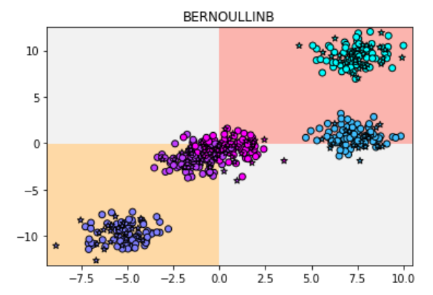
It seems that Bayes effort naive Bayes is really only suitable for the classification task of 0-1 variables.

3.2 Gaussian naive Bayes

Then Gaussian naive Bayes classification

#Gauss naive Bayes
from sklearn.naive_bayes import GaussianNB
gnb=GaussianNB()
gnb.fit(x_train,y_train)
gnb.score(x_test,y_test)
#Draw a picture
z=gnb.predict(np.c_[(xx.ravel(),yy.ravel())]).reshape(xx.shape)
plt.pcolormesh(xx,yy,z,cmap=plt.cm.Pastel1)
#The test set and training set are represented by scatter diagram
plt.scatter(x_train[:,0],x_train[:,1],c=y_train,cmap=plt.cm.cool,edgecolor='k')
plt.scatter(x_test[:,0],x_test[:,1],c=y_test,cmap=plt.cm.cool,marker="*",edgecolor="k")
plt.xlim(xx.min(),xx.max())
plt.ylim(yy.min(),yy.max())
plt.title("gaussianNB")
plt.show()

The result is: the accuracy is 0.968, super high

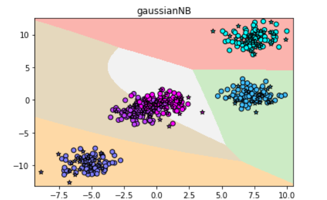
It seems that Gaussian distribution is very suitable for this data set

3.3 polynomial naive Bayes

Let's look at polynomial naive Bayes

#Classification using polynomial naive Bayes
from sklearn.naive_bayes import MultinomialNB
#Polynomial naive Bayes is used to fit the data
mnb=MultinomialNB()
mnb.fit(x_train,y_train)
mnb.score(x_test,y_test)

Direct error reporting: the display x cannot be negative

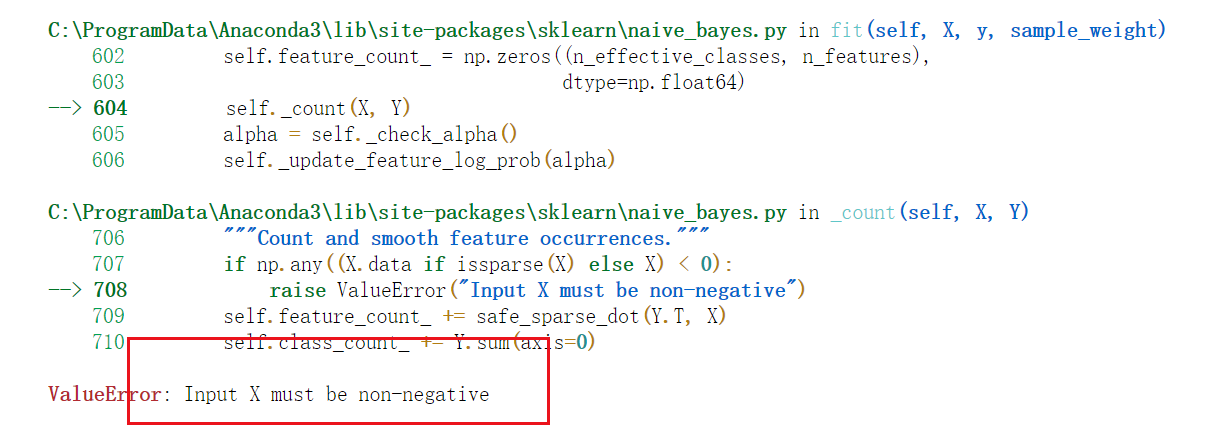
Polynomial naive Bayes is only suitable for the classification of non negative discrete numerical features. The data here has negative values, so it is not suitable for this method.

4. Case analysis

In fact, Gaussian naive Bayes is the most commonly used in Bayes, because a large number of phenomena in the fields of natural sciences and Social Sciences conform to the law of normal distribution, and Gaussian naive Bayes can be competent for most classification tasks.
We classify the tumor data set in sklearn, which contains 569 sample data and 30 eigenvalues. Let's see the effect.

• Import dataset

#Let's look at the form of data sets
from sklearn.datasets import load_breast_cancer
cancer=load_breast_cancer()
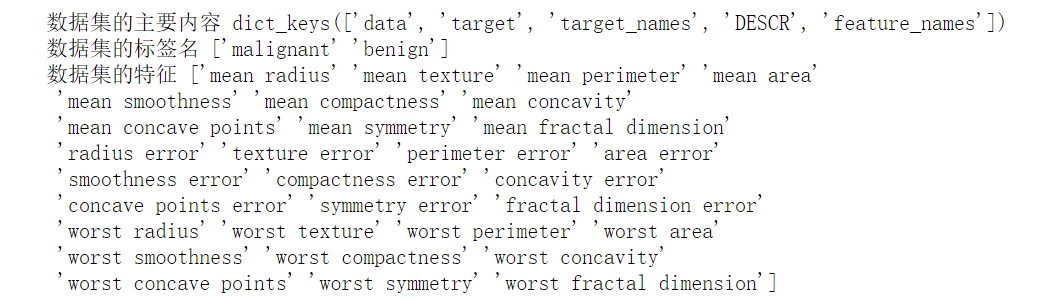
print("Main contents of data set",cancer.keys())
print("Label name of the dataset",cancer["target_names"])
print("Characteristics of data sets",cancer["feature_names"])

The results are as follows:

• Partition dataset

#Divide the dataset into x and y
x,y=cancer.data,cancer.target
#Split training set and test set using data set
x_train,x_test,y_train,y_test=train_test_split(x,y,random_state=38)
print("Training set form;",x_train.shape)
print("Test set data form:",x_test.shape)

The results are as follows:

• Gaussian Bayesian fitting

gnb=GaussianNB()
gnb.fit(x_train,y_train)
print("Test set score:",gnb.score(x_train,y_train))
print("Training set score:",gnb.score(x_test,y_test))

The results are as follows:

reference material

python machine learning in simple terms
Statistical learning methods