neuron
Neuron and perceptron are essentially the same, but when we say perceptron, its activation function is a step function; When we talk about neurons, the activation function is often sigmoid function or tanh function. As shown in the figure below: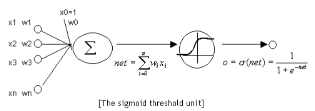
The method of calculating the output of a neuron is the same as that of a perceptron. Suppose the input of a neuron is a vector , the weight vector is
 (the offset term is
  ), if the activation function is a sigmoid function, its output
 :
:

The sigmoid function is defined as follows:

Take it into the previous equation and get

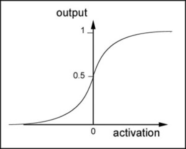
sigmoid function is a nonlinear function with a range of (0,1). The function image is shown in the figure below
The derivative of sigmoid function is:

As you can see, the derivative of sigmoid function is very interesting. It can be expressed by sigmoid function itself. In this way, once the value of sigmoid function is calculated, it is very convenient to calculate the value of its derivative.
What is neural network
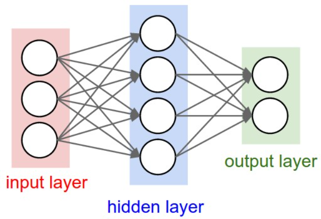
Neural network is actually a number of neurons connected according to certain rules. The figure above shows a fully connected (FC) neural network. By observing the figure above, we can find that its rules include:
- Neurons are arranged in layers. The leftmost layer is called the input layer, which is responsible for receiving input data; The rightmost layer is called the output layer, from which we can obtain the output data of neural network. The layers between the input layer and the output layer are called hidden layers because they are invisible to the outside.
- There is no connection between neurons in the same layer.
- Each neuron in layer N is connected to all neurons in layer N-1 (this is the meaning of full connected), and the output of neurons in layer N-1 is the input of neurons in layer n.
- Each connection has a weight.
These rules define the structure of fully connected neural networks. In fact, there are many other neural networks, such as convolutional neural network (CNN) and cyclic neural network (RNN), which have different connection rules.
Calculate the output of neural network
Neural network is actually an input vector To output vector
 Functions of, i.e.:

To calculate the output of the neural network according to the input, we need to first convert the input vector Each element of
 The value of is assigned to the corresponding neurons of the input layer of the neural network, and then the value of each neuron of each layer is calculated forward according to equation 1 until the value of all neurons of the output layer of the last layer is calculated. Finally, the output vector is obtained by concatenating the values of each neuron in the output layer
 .
.
Next, take an example to illustrate this process. We first write the number of each unit of the neural network.
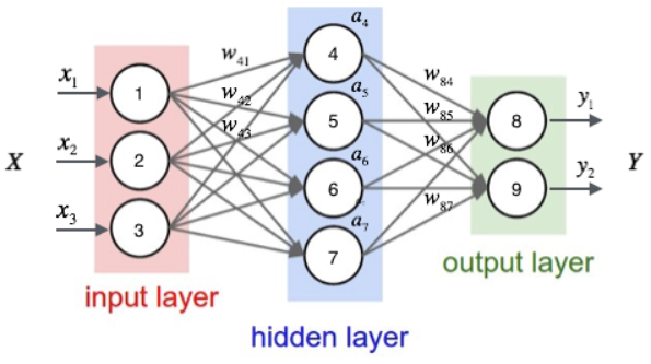
As shown in the figure above, the input layer has three nodes, which are numbered as 1, 2 and 3 in turn; The 4 nodes of the hidden layer are numbered 4, 5, 6 and 7; Finally, the two nodes of the output layer are numbered 8 and 9. Because our neural network is a fully connected network, we can see that each node is connected to all nodes in the upper layer. For example, we can see that node 4 of the hidden layer is connected with three nodes 1, 2 and 3 of the input layer, and the weight of the connection is . So, how do we calculate the output value of node 4
 And?
And?
In order to calculate the output value of node 4, we must first obtain the output values of all its upstream nodes (i.e. nodes 1, 2 and 3). Nodes 1, 2 and 3 are the nodes of the input layer, so their output values are the input vectors Itself. According to the corresponding relationship shown in the figure above, you can see that the output values of nodes 1, 2 and 3 are
 . We require that the dimension of the input vector is the same as the number of neurons in the input layer, and the input node corresponding to an element of the input vector can be determined freely. You don't want to
 There is no problem with assigning a value to node 2, but it is of little value except to stun yourself.
Once we have the output values of nodes 1, 2 and 3, we can calculate the output value of node 4 according to equation 1 :
:

Above formula Is the offset term of node 4, which is not drawn in the figure. and
 These are the weights connected from node 1, 2 and 3 to node 4 respectively
 When numbering, we put the number of the target node
 Put it first and put the number of the source node
 Put it in the back.
Similarly, we can continue to calculate the output values of nodes 5, 6 and 7 . In this way, the output values of the four nodes of the hidden layer are calculated, and we can then calculate the output values of node 8 of the output layer
 :
:

Similarly, we can also calculate Value of. In this way, the output values of all nodes in the output layer are calculated, and we get the input vector
 The output vector of the neural network
 . Here we also see that the dimension of the output vector is the same as the number of neurons in the output layer.
Matrix representation of neural networks
The calculation of neural network will be very convenient if it is represented by matrix (of course, the lattice is higher). Let's first look at the matrix representation of hidden layer.
First, we arrange the calculations of the four nodes of the hidden layer in turn:

Next, the input vector of the network is defined And the weight vector of each node of the hidden layer
 . order

Substitute into the previous set of equations to obtain:

Now, let's put the above calculation The four formulas of are written into a matrix. Each formula is used as a row of the matrix, and their calculation can be expressed by the matrix. order

Bring in the previous set of equations and get

In equation 2, Is the activation function, in this case, the sigmoid function;
 Is the weight matrix of a layer;
 Is the input vector of a layer;
 Is the output vector of a layer. Equation 2 shows that the function of each layer of neural network is actually to multiply the input vector left by an array for linear transformation to obtain a new vector, and then apply an activation function to this vector element by element.
The algorithm of each layer is the same. For example, for neural networks with one input layer, one output layer and three hidden layers, we assume that their weight matrices are , the output of each hidden layer is
 , the input of neural network is
 , the input of neural network is
 , as shown in the figure below:
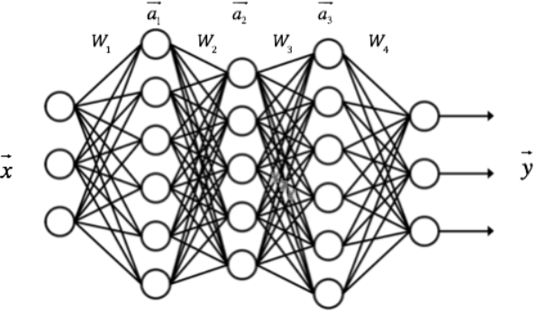
Then the calculation of the output vector of each layer can be expressed as:
 This is the calculation method of the output value of neural network.
Training of neural network
Now, we need to know how to get the weight on each connection of a neural network. We can say that neural network is a model, so these weights are the parameters of the model, that is, what the model needs to learn. However, the connection mode, the number of layers and the number of nodes in each layer of a neural network are not learned, but artificially set in advance. These artificially set parameters are called hyper parameters.
Next, we will introduce the training algorithm of neural network: back propagation algorithm.
Back propagation algorithm
We first intuitively introduce the back propagation algorithm, and finally introduce the derivation of this algorithm. Of course, readers can skip the derivation part completely, because even if you don't know how to deduce, it doesn't affect you to write the training code of a neural network. In fact, there are many mature open source implementations of neural networks. Except for practicing, you may not have the opportunity to write a neural network.
We take supervised learning as an example to explain the back propagation algorithm. stay Zero basis introduction to deep learning (2) - linear units and gradient descent In this article, we introduced what supervised learning is. If you forget it, you can take a look again. In addition, we set the activation function of neurons Is a function (the calculation formulas of different activation functions are different, see Derivation of back propagation algorithm Section).
We assume that each training sample is Where vector
 Is the characteristic of the training sample, and
 Is the target value of the sample.
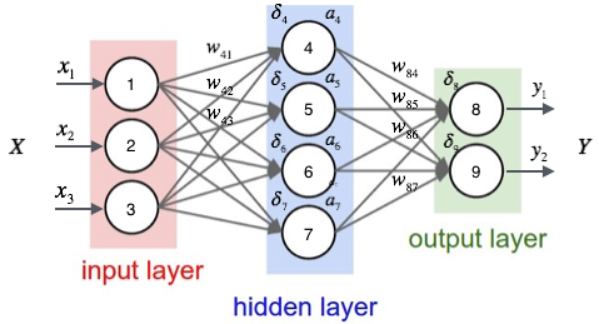
Firstly, we use the characteristics of samples according to the algorithm introduced in the previous section , the output of each hidden layer node in the neural network is calculated
  And the output of each node of the output layer
 .
.
Then, we calculate the error term of each node according to the following method :
:
- For output layer nodes
 ,
,

Among them, Is the error term of the node,
 Is node
 Output value of,
  Yes, the sample corresponds to the node
 Target value for. For example, according to the above figure, for the output layer node 8, its output value is
 , and the target value of the sample is
 , bring in the above formula to obtain the error term of node 8
 Should be:

- For hidden layer nodes,

Among them, Is node
 Output value of,
 Is node
 To its next level node
 The weight of the connection,
 Is node
 Next level node
 Error term. For example, for hidden layer node 4, the calculation method is as follows:

Finally, update the weights on each connection:

Among them, Is node
 To node
 The weight of,
 Is a constant that becomes the learning rate,
 Is node
 Error term,
 Is node
  Pass to node
 Input of. For example, weights
 The update method is as follows:

Similarly, weight The update method is as follows:

The input value of the offset item is always 1. For example, the offset term of node 4 It shall be calculated as follows:

We have introduced the calculation and weight update method of each node error term of neural network. Obviously, to calculate the error term of a node, we need to calculate the error term of each node connected to the next layer. This requires that the calculation order of the error term must start from the output layer, and then calculate the error term of each hidden layer in reverse order until the hidden layer connected to the input layer. This is the meaning of the name of the back propagation algorithm. When the error terms of all nodes are calculated, we can update all weights according to equation 5.
The above is the basic back propagation algorithm, which is not very complex. Have you figured it out?
Derivation of back propagation algorithm
Back propagation algorithm is actually the application of chain derivation rule. However, this simple and obvious method was invented and popularized nearly 30 years after Roseblatt proposed the perceptron algorithm. In response, Bengio responded:
Many seemingly obvious ideas become obvious only after the fact.
Next, we use the chain derivation rule to derive the back propagation algorithm, that is, equations 3, 4 and 5 in the previous section.
High energy early warning ahead - next is the hardest hit area of mathematical formula. Readers can read it at their own discretion without forcing.
According to the general routine of machine learning, we first determine the objective function of the neural network, and then use the random gradient descent optimization algorithm to find the parameter value when the minimum value of the objective function is obtained.
We take the sum of squares of errors of all output layer nodes of the network as the objective function:

Among them, Indicates a sample
 Error.
Then, we use the article Zero basis introduction to deep learning (2) - linear units and gradient descent The random gradient descent algorithm introduced in optimizes the objective function:

The random gradient descent algorithm needs to find the error For each weight
 How do you find the partial derivative of (that is, the gradient)?
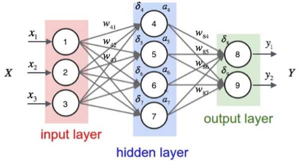
Looking at the figure above, we find that the weight Only by affecting nodes
 The input value of affects other parts of the network
 Is node
 Weighted input, i.e

 yes
yes Function, and
 yes
yes Function of. According to the chain derivation rule, we can get:

Where, Is node
 Pass to node
 The input value of the node, that is, the output value of the node.
about It is necessary to distinguish between output layer and hidden layer.
Output layer weight training
For the output layer, Only through nodes
 Output value of
 To affect the rest of the network, that is
 yes
yes Function, and
 yes
yes Function of, where
 . So we can use the chain derivation rule again:

Consider the first item of the above formula:

Consider the second item of the above formula:

Bring in the first and second items to get:

If order That is, the error term of a node
 Is the inverse of the partial derivative of the network error to the input of this node. Bring in the above formula to obtain:

The above formula is formula 3.
The above derivation is brought into the random gradient descent formula to obtain:

The above equation is equation 5.
Hidden layer weight training
Now we're going to derive the of the hidden layer .
.
First, we need to define nodes A collection of all direct downstream nodes
 . For example, for node 4, its direct downstream nodes are node 8 and node 9. Can see
 Only through influence
 Re influence
 . set up
 Is node
 The input of the downstream node, then
 yes
yes Function, and
 yes
yes Function of. because
 There are several. We can make the following derivation by using the full derivative formula:
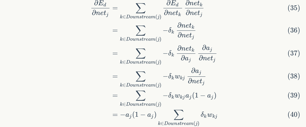
because , bring in the above formula to obtain:

The above equation is equation 4.
——Math formula alarm cleared——
So far, we have derived the back propagation algorithm. It should be noted that the training rules we just deduced are based on the activation function is sigmoid function, square sum error, fully connected network and random gradient descent optimization algorithm. If the activation function is different, the error calculation method is different, the network connection structure is different, and the optimization algorithm is different, the specific training rules will be different. However, in any case, the derivation of training rules is the same, which can be deduced by using the chain derivation rule.
Implementation of neural network
For the complete code, please refer to GitHub: https://github.com/hanbt/learn_dl/blob/master/bp.py (python2.7)
Now, we need to implement a basic fully connected neural network according to the previous algorithm, which does not require much code. We still use object-oriented design here.
First, let's make a basic model:
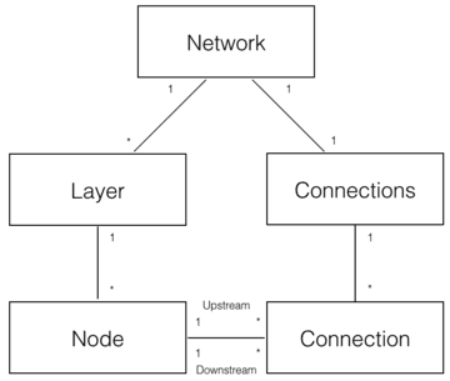
As shown in the figure above, five domain objects can be decomposed to realize the neural network:
- Network neural network object, which provides API interface. It consists of several layer objects and connected objects.
- A Layer object that consists of multiple nodes.
- The Node object calculates and records the Node's own information (such as output values)
 . error term
 And the upstream and downstream connections associated with this node.
 - Connection each connection object should record the weight of the connection.
- Connections only serves as the collection object of Connection and provides some collection operations.
Node implementation is as follows:
# The node class is responsible for recording and maintaining the node's own information and the upstream and downstream connections related to this node, and realizing the calculation of output value and error term.
2.class Node(object):
3.    def __init__(self, layer_index, node_index):
4.        '''
5.        Construct node objects.
6.        layer_index: The number of the layer to which the node belongs
7.        node_index: Node number
8.        '''
9.        self.layer_index = layer_index
10.        self.node_index = node_index
11.        self.downstream = []
12.        self.upstream = []
13.        self.output = 0
14.        self.delta = 0
15.
16.    def set_output(self, output):
17.        '''
18.        Sets the output value of the node. This function is used if the node belongs to the input layer.
19.        '''
20.        self.output = output
21.
22.    def append_downstream_connection(self, conn):
23.        '''
24.        Add a connection to the downstream node
25.        '''
26.        self.downstream.append(conn)
27.
28.    def append_upstream_connection(self, conn):
29.        '''
30.        Add a connection to the upstream node
31.        '''
32.        self.upstream.append(conn)
33.
34.    def calc_output(self):
35.        '''
36.        Calculate the output of the node according to equation 1
37.        '''
38.        output = reduce(lambda ret, conn: ret + conn.upstream_node.output * conn.weight, self.upstream, 0)
39.        self.output = sigmoid(output)
40.
41.    def calc_hidden_layer_delta(self):
42.        '''
43.        When the node belongs to the hidden layer, it is calculated according to equation 4 delta
44.        '''
45.        downstream_delta = reduce(
46.            lambda ret, conn: ret + conn.downstream_node.delta * conn.weight,
47.            self.downstream, 0.0)
48.        self.delta = self.output * (1 - self.output) * downstream_delta
49.
50.    def calc_output_layer_delta(self, label):
51.        '''
52.        When the node belongs to the output layer, it is calculated according to equation 3 delta
53.        '''
54.        self.delta = self.output * (1 - self.output) * (label - self.output)
55.
56.    def __str__(self):
57.        '''
58.        Print node information
59.        '''
60.        node_str = '%u-%u: output: %f delta: %f' % (self.layer_index, self.node_index, self.output, self.delta)
61.        downstream_str = reduce(lambda ret, conn: ret + '\n\t' + str(conn), self.downstream, '')
62.        upstream_str = reduce(lambda ret, conn: ret + '\n\t' + str(conn), self.upstream, '')
63.        return node_str + '\n\tdownstream:' + downstream_str + '\n\tupstream:' + upstream_str
ConstNode object, in order to realize a node whose output is constant 1 (calculate the offset term (if required)
class ConstNode(object):
2.    def __init__(self, layer_index, node_index):
3.        '''
4.        Construct node objects.
5.        layer_index: The number of the layer to which the node belongs
6.        node_index: Node number
7.        '''
8.        self.layer_index = layer_index
9.        self.node_index = node_index
10.        self.downstream = []
11.        self.output = 1
12.
13.    def append_downstream_connection(self, conn):
14.        '''
15.        Add a connection to the downstream node
16.        '''
17.        self.downstream.append(conn)
18.
19.    def calc_hidden_layer_delta(self):
20.        '''
21.        When the node belongs to the hidden layer, it is calculated according to equation 4 delta
22.        '''
23.        downstream_delta = reduce(
24.            lambda ret, conn: ret + conn.downstream_node.delta * conn.weight,
25.            self.downstream, 0.0)
26.        self.delta = self.output * (1 - self.output) * downstream_delta
27.
28.    def __str__(self):
29.        '''
30.        Print node information
31.        '''
32.        node_str = '%u-%u: output: 1' % (self.layer_index, self.node_index)
33.        downstream_str = reduce(lambda ret, conn: ret + '\n\t' + str(conn), self.downstream, '')
34.        return node_str + '\n\tdownstream:' + downstream_str
Layer object, which is responsible for initializing a layer. In addition, as a collection object of nodes, it provides operations on Node collections.
class Layer(object):
2.    def __init__(self, layer_index, node_count):
3.        '''
4.        Initialize layer 1
5.        layer_index: Layer number
6.        node_count: Number of nodes contained in the layer
7.        '''
8.        self.layer_index = layer_index
9.        self.nodes = []
10.        for i in range(node_count):
11.            self.nodes.append(Node(layer_index, i))
12.        self.nodes.append(ConstNode(layer_index, node_count))
13.
14.    def set_output(self, data):
15.        '''
16.        Sets the output of the layer. Used when the layer is an input layer.
17.        '''
18.        for i in range(len(data)):
19.            self.nodes[i].set_output(data[i])
20.
21.    def calc_output(self):
22.        '''
23.        Calculate the output vector of the layer
24.        '''
25.        for node in self.nodes[:-1]:
26.            node.calc_output()
27.
28.    def dump(self):
29.        '''
30.        Print layer information
31.        '''
32.        for node in self.nodes:
33.            print node
The Connection object is mainly responsible for recording the weight of the Connection and the upstream and downstream nodes associated with the Connection.
class Connection(object):
2.    def __init__(self, upstream_node, downstream_node):
3.        '''
4.        Initialize the connection. The weight is initialized to a small random number
5.        upstream_node: Connected upstream node
6.        downstream_node: Connected downstream nodes
7.        '''
8.        self.upstream_node = upstream_node
9.        self.downstream_node = downstream_node
10.        self.weight = random.uniform(-0.1, 0.1)
11.        self.gradient = 0.0
12.
13.    def calc_gradient(self):
14.        '''
15.        Calculated gradient
16.        '''
17.        self.gradient = self.downstream_node.delta * self.upstream_node.output
18.
19.    def get_gradient(self):
20.        '''
21.        Gets the current gradient
22.        '''
23.        return self.gradient
24.
25.    def update_weight(self, rate):
26.        '''
27.        Update the weight according to the gradient descent algorithm
28.        '''
29.        self.calc_gradient()
30.        self.weight += rate * self.gradient
31.
32.    def __str__(self):
33.        '''
34.        Print connection information
35.        '''
36.        return '(%u-%u) -> (%u-%u) = %f' % (
37.            self.upstream_node.layer_index,
38.            self.upstream_node.node_index,
39.            self.downstream_node.layer_index,
40.            self.downstream_node.node_index,
41.            self.weight)
Connections object that provides Connection collection operations.
class Connections(object):
2.    def __init__(self):
3.        self.connections = []
4.
5.    def add_connection(self, connection):
6.        self.connections.append(connection)
7.
8.    def dump(self):
9.        for conn in self.connections:
10.            print conn
Network object that provides API s.
class Network(object):
2.    def __init__(self, layers):
3.        '''
4.        Initialize a fully connected neural network
5.        layers: A two-dimensional array describing the number of nodes in each layer of the neural network
6.        '''
7.        self.connections = Connections()
8.        self.layers = []
9.        layer_count = len(layers)
10.        node_count = 0;
11.        for i in range(layer_count):
12.            self.layers.append(Layer(i, layers[i]))
13.        for layer in range(layer_count - 1):
14.            connections = [Connection(upstream_node, downstream_node)
15.                           for upstream_node in self.layers[layer].nodes
16.                           for downstream_node in self.layers[layer + 1].nodes[:-1]]
17.            for conn in connections:
18.                self.connections.add_connection(conn)
19.                conn.downstream_node.append_upstream_connection(conn)
20.                conn.upstream_node.append_downstream_connection(conn)
21.
22.
23.    def train(self, labels, data_set, rate, iteration):
24.        '''
25.        Training neural network
26.        labels: Array, training sample label. Each element is a label of a sample.
27.        data_set: Two dimensional array, training sample features. Each element is a feature of a sample.
28.        '''
29.        for i in range(iteration):
30.            for d in range(len(data_set)):
31.                self.train_one_sample(labels[d], data_set[d], rate)
32.
33.    def train_one_sample(self, label, sample, rate):
34.        '''
35.        The internal function uses a sample to train the network
36.        '''
37.        self.predict(sample)
38.        self.calc_delta(label)
39.        self.update_weight(rate)
40.
41.    def calc_delta(self, label):
42.        '''
43.        Internal function to calculate the of each node delta
44.        '''
45.        output_nodes = self.layers[-1].nodes
46.        for i in range(len(label)):
47.            output_nodes[i].calc_output_layer_delta(label[i])
48.        for layer in self.layers[-2::-1]:
49.            for node in layer.nodes:
50.                node.calc_hidden_layer_delta()
51.
52.    def update_weight(self, rate):
53.        '''
54.        Internal function to update the weight of each connection
55.        '''
56.        for layer in self.layers[:-1]:
57.            for node in layer.nodes:
58.                for conn in node.downstream:
59.                    conn.update_weight(rate)
60.
61.    def calc_gradient(self):
62.        '''
63.        Internal function to calculate the gradient of each connection
64.        '''
65.        for layer in self.layers[:-1]:
66.            for node in layer.nodes:
67.                for conn in node.downstream:
68.                    conn.calc_gradient()
69.
70.    def get_gradient(self, label, sample):
71.        '''
72.        Obtain the gradient on each connection of the network under one sample
73.        label: Sample label
74.        sample: Sample input
75.        '''
76.        self.predict(sample)
77.        self.calc_delta(label)
78.        self.calc_gradient()
79.
80.    def predict(self, sample):
81.        '''
82.        Predict the output value according to the input sample
83.        sample: Array, the characteristics of the sample, that is, the input vector of the network
84.        '''
85.        self.layers[0].set_output(sample)
86.        for i in range(1, len(self.layers)):
87.            self.layers[i].calc_output()
88.        return map(lambda node: node.output, self.layers[-1].nodes[:-1])
89.
90.    def dump(self):
91.        '''
92.        Print network information
93.        '''
94.        for layer in self.layers:
95.            layer.dump()
Gradient check
How to ensure that the neural network you write has no BUG? In fact, this is a very important issue. On the one hand, I have worked hard to think of an algorithm, and the result is not ideal. Is the algorithm itself wrong or the code implementation wrong? Locating this problem must take a lot of time and energy. On the other hand, due to the complexity of neural network, we can hardly know the input and output of neural network in advance. Therefore, development methods such as TDD (Test Driven Development) seem to be infeasible.
The way is to use gradient check to confirm whether the program is correct. The idea of gradient inspection is as follows:
For gradient descent algorithm:

The key here is The calculation must be correct, and it is
 yes
yes Partial derivative of. According to the definition of derivative:

For any We can use the right side of the equation to approximate the derivative of. We put
 yes
yes Function of, i.e
 So, according to the derivative definition,
 Should be equal to:

If you put Set to a small number (e.g
 ), then the above formula can be written as:

We can use equation 6 to calculate the gradient And then compare it with the gradient value calculated in our neural network code. If the difference between the two is very small, then our code is correct.
The following is the code for gradient check. If we want to check the parameters Whether the gradient is correct, we need the following steps:
- Firstly, a sample is used to train the neural network, so that the gradient of each weight can be obtained.
- A small value () will be added to recalculate the neural network under this sample.
- A small value () will be subtracted to recalculate the neural network under this sample.
- Calculate the desired gradient value according to equation 6 and compare it with the gradient value obtained in the first step. They should be almost equal (at least 4 significant digits are the same).
Of course, we can repeat the above process to check each weight. Multiple samples can also be used to repeat the inspection.
def gradient_check(network, sample_feature, sample_label):
2.    '''
3.    Gradient check
4.    network: Neural network object
5.    sample_feature: Characteristics of samples
6.    sample_label: Label of sample
7.    '''
8.    # Calculate network error
9.    network_error = lambda vec1, vec2: \
10.            0.5 * reduce(lambda a, b: a + b,
11.                      map(lambda v: (v[0] - v[1]) * (v[0] - v[1]),
12.                          zip(vec1, vec2)))
13.
14.    # Get the gradient of each connection of the network under the current sample
15.    network.get_gradient(sample_feature, sample_label)
16.
17.    # Gradient check for each weight
18.    for conn in network.connections.connections:
19.        # Gets the gradient of the specified connection
20.        actual_gradient = conn.get_gradient()
21.
22.        # Add a small value to calculate the error of the network
23.        epsilon = 0.0001
24.        conn.weight += epsilon
25.        error1 = network_error(network.predict(sample_feature), sample_label)
26.
27.        # Subtract a small value to calculate the error of the network
28.        conn.weight -= 2 * epsilon # I just added it once, so I need to subtract twice here
29.        error2 = network_error(network.predict(sample_feature), sample_label)
30.
31.        # Calculate the desired gradient value according to equation 6
32.        expected_gradient = (error2 - error1) / (2 * epsilon)
33.
34.        # Print
35.        print 'expected gradient: \t%f\nactual gradient: \t%f' % (
36.            expected_gradient, actual_gradient)
Neural network practice -- handwritten numeral recognition
For this task, we use the MNIST dataset, which is very popular in the industry. MNIST has about 60000 training samples of handwritten letters. We use it to train our neural network, and then use the trained network to recognize handwritten digits.
Handwritten numeral recognition is a relatively simple task. Numbers can only be one of 0-9, which is a 10 classification problem.
Determination of super parameters
We first need to determine the number of layers of the network and the number of nodes in each layer. As for the first question, in fact, there is no theoretical method. Everyone takes pictures based on experience. If there is no experience, just take one at random. Then, you can try a few more values and train neural networks with different layers to see which one works best. Well, now you may understand why deep learning is a craft. Some crafts are speechless, while others are very technical.
However, we still understand some basic principles. We know that the more layers of the network, the better. We also know that the more layers, the more difficult it is to train. For fully connected networks, the hidden layer should not exceed three layers. Then, we can first try the effect of neural network with only one hidden layer. After all, if the model is small, the training is faster (when I first started playing the model, I hope to see the results quickly).
The number of input layer nodes is determined. Because each training data of MNIST dataset is a 28 * 28 picture with a total of 784 pixels, the number of input layer nodes should be 784, and each pixel corresponds to an input node.
The number of output layer nodes is also determined. Because it is 10 classification, we can use 10 nodes, and each node corresponds to a classification. Among the 10 nodes in the output layer, the classification corresponding to the node that outputs the maximum value is the prediction result of the model.
The number of hidden layer nodes is uncertain, ranging from 1 to 1 million. Here are several empirical formulas:

Therefore, we can first set the number of hidden layer nodes according to the above formula. If we have time, we can set different node numbers and train them separately to see which effect is the best. Let's take one first and set the number of hidden layer nodes to 300.
For 3 layers All connected network, a total of
 Parameters! The reason why neural network is powerful is that it provides a very simple method to realize a large number of parameters. At present, there are also super large-scale neural networks with 10 billion parameters and 100 billion samples. Because MNIST has only 60000 training samples, too many parameters are easy to fit, but the effect is not good.
Model training and evaluation
The MNIST dataset contains 10000 test samples. We first train our network with 60000 training samples, and then test the network with test samples to calculate the recognition error rate:

We evaluate the accuracy every 10 rounds of training. When the accuracy begins to decline (over fitting occurs), the training is terminated.
code implementation
First, we need to process the MNIST data set into a form acceptable to the neural network. The file format of MNIST training set can refer to the official website, which will not be repeated here. Each training sample is a 28 * 28 image. We convert it into a 784 dimensional vector according to row priority. Each label is a value of 0-9. We convert it into a 10 dimensional one hot vector: if the label value is, we set the dimension of the vector (numbered from 0) to 0.9 and the other dimensions to 0.1. For example, the vector [0.1,0.1,0.9,0.1,0.1,0.1,0.1,0.1,0.1,0.1,0.1] represents the value 2.
The following is the code for processing MNIST data:
#!/usr/bin/env python
2.# -*- coding: UTF-8 -*-
3.
4.import struct
5.from bp import *
6.from datetime import datetime
7.
8.
9.# Data loader base class
10.class Loader(object):
11.    def __init__(self, path, count):
12.        '''
13.        Initialize loader
14.        path: Data file path
15.        count: Number of samples in the file
16.        '''
17.        self.path = path
18.        self.count = count
19.
20.    def get_file_content(self):
21.        '''
22.        Read file contents
23.        '''
24.        f = open(self.path, 'rb')
25.        content = f.read()
26.        f.close()
27.        return content
28.
29.    def to_int(self, byte):
30.        '''
31.        take unsigned byte Convert characters to integers
32.        '''
33.        return struct.unpack('B', byte)[0]
34.
35.
36.# Image data loader
37.class ImageLoader(Loader):
38.    def get_picture(self, content, index):
39.        '''
40.        Internal function to obtain an image from a file
41.        '''
42.        start = index * 28 * 28 + 16
43.        picture = []
44.        for i in range(28):
45.            picture.append([])
46.            for j in range(28):
47.                picture[i].append(
48.                    self.to_int(content[start + i * 28 + j]))
49.        return picture
50.
51.    def get_one_sample(self, picture):
52.        '''
53.        Internal function to convert the image into the input vector of the sample
54.        '''
55.        sample = []
56.        for i in range(28):
57.            for j in range(28):
58.                sample.append(picture[i][j])
59.        return sample
60.
61.    def load(self):
62.        '''
63.        Load the data file to obtain the input vector of all samples
64.        '''
65.        content = self.get_file_content()
66.        data_set = []
67.        for index in range(self.count):
68.            data_set.append(
69.                self.get_one_sample(
70.                    self.get_picture(content, index)))
71.        return data_set
72.
73.
74.# Tag data loader
75.class LabelLoader(Loader):
76.    def load(self):
77.        '''
78.        Load the data file to obtain the label vector of all samples
79.        '''
80.        content = self.get_file_content()
81.        labels = []
82.        for index in range(self.count):
83.            labels.append(self.norm(content[index + 8]))
84.        return labels
85.
86.    def norm(self, label):
87.        '''
88.        Internal function to convert a value into a 10 dimensional label vector
89.        '''
90.        label_vec = []
91.        label_value = self.to_int(label)
92.        for i in range(10):
93.            if i == label_value:
94.                label_vec.append(0.9)
95.            else:
96.                label_vec.append(0.1)
97.        return label_vec
98.
99.
100.def get_training_data_set():
101.    '''
102.    Obtain training data set
103.    '''
104.    image_loader = ImageLoader('train-images-idx3-ubyte', 60000)
105.    label_loader = LabelLoader('train-labels-idx1-ubyte', 60000)
106.    return image_loader.load(), label_loader.load()
107.
108.
109.def get_test_data_set():
110.    '''
111.    Get test data set
112.    '''
113.    image_loader = ImageLoader('t10k-images-idx3-ubyte', 10000)
114.    label_loader = LabelLoader('t10k-labels-idx1-ubyte', 10000)
115.    return image_loader.load(), label_loader.load()
The output of the network is a 10 dimensional vector. If the value of the first (numbered from 0) element of this vector is the largest, it is the recognition result of the network. The following is the code implementation:
def get_result(vec):
2.    max_value_index = 0
3.    max_value = 0
4.    for i in range(len(vec)):
5.        if vec[i] > max_value:
6.            max_value = vec[i]
7.            max_value_index = i
8.    return max_value_index
We use the error rate to evaluate the network. The following is the code implementation:
def evaluate(network, test_data_set, test_labels):
2.    error = 0
3.    total = len(test_data_set)
4.
5.    for i in range(total):
6.        label = get_result(test_labels[i])
7.        predict = get_result(network.predict(test_data_set[i]))
8.        if label != predict:
9.            error += 1
10.    return float(error) / float(total)
Finally, we implement our training strategy: evaluate the accuracy once every 10 rounds of training, and terminate the training when the accuracy begins to decline. The following is the code implementation:
def train_and_evaluate():
2.    last_error_ratio = 1.0
3.    epoch = 0
4.    train_data_set, train_labels = get_training_data_set()
5.    test_data_set, test_labels = get_test_data_set()
6.    network = Network([784, 300, 10])
7.    while True:
8.        epoch += 1
9.        network.train(train_labels, train_data_set, 0.3, 1)
10.        print '%s epoch %d finished' % (now(), epoch)
11.        if epoch % 10 == 0:
12.            error_ratio = evaluate(network, test_data_set, test_labels)
13.            print '%s after epoch %d, error ratio is %f' % (now(), epoch, error_ratio)
14.            if error_ratio > last_error_ratio:
15.                break
16.            else:
17.                last_error_ratio = error_ratio
18.
19.
20.if __name__ == '__main__':
21.    train_and_evaluate()
I tested it on my machine. An epoch takes about 9000 seconds, Therefore, we need to do a lot of performance optimization for the code (such as vector programming). The training takes a long time. You can upload it to the server and run it in the tmux session. In order to prevent the previous work from being wasted due to abnormal termination, we save the obtained parameter values on the disk every 10 rounds of training so that they can be recovered later. (code omitted)
Vectorization programming
For the complete code, please refer to GitHub: https://github.com/hanbt/learn_dl/blob/master/fc.py (python2.7)
After a long training, we may think that there must be a better way! Yes, programmers, now we need to say goodbye to object-oriented programming and use another programming method more suitable for deep learning algorithm: vectorial programming. There are two main reasons: one is that we don't really need to define objects such as Node and Connection, so we can directly implement mathematical calculation; Another reason, It is the underlying algorithm library that will optimize vector operations (even special hardware, such as GPU), and the program efficiency will be greatly improved. Therefore, in the world of deep learning, we will always try to express the calculation in the form of vectors. I believe that excellent programmers will not stick to a certain way (familiar with) programming paradigm, but will learn and use the most appropriate paradigm.
Next, we use the vector programming method to re implement the previous fully connected neural network.
First, we need to express all the calculations in the form of vectors. For fully connected neural networks, there are three main calculation formulas.
For forward calculation, we find that equation 2 is already a vectorized expression:

In the above formula Represents the sigmoid function.
For reverse calculation, we need to use vectors to express Equations 3 and 4:

In equation 8, Represents the error term of layer l;
 Representation matrix
 Transpose of.
We also need a vectorized representation of the gradient calculation of the weight array W and the bias term b. That is, equation 5 needs to be expressed by vectorization:

The corresponding vectorization is expressed as:

The vectorization of the update offset term is expressed as:

Now, according to the above formulas, we re implement a class: FullConnectedLayer. It realizes the forward and backward calculation of the full connection layer:
# Full connection layer implementation class
2.class FullConnectedLayer(object):
3.    def __init__(self, input_size, output_size,
4.                 activator):
5.        '''
6.        Constructor
7.        input_size: Dimension of input vector of this layer
8.        output_size: Dimension of output vector of this layer
9.        activator: Activation function
10.        '''
11.        self.input_size = input_size
12.        self.output_size = output_size
13.        self.activator = activator
14.        # Weight array W
15.        self.W = np.random.uniform(-0.1, 0.1,
16.            (output_size, input_size))
17.        # Offset term b
18.        self.b = np.zeros((output_size, 1))
19.        # Output vector
20.        self.output = np.zeros((output_size, 1))
21.
22.    def forward(self, input_array):
23.        '''
24.        Forward calculation
25.        input_array: Input vector, dimension must be equal to input_size
26.        '''
27.        # Equation 2
28.        self.input = input_array
29.        self.output = self.activator.forward(
30.            np.dot(self.W, input_array) + self.b)
31.
32.    def backward(self, delta_array):
33.        '''
34.        Reverse calculation W and b Gradient of
35.        delta_array: Error term passed from the upper layer
36.        '''
37.        # Equation 8
38.        self.delta = self.activator.backward(self.input) * np.dot(
39.            self.W.T, delta_array)
40.        self.W_grad = np.dot(delta_array, self.input.T)
41.        self.b_grad = delta_array
42.
43.    def update(self, learning_rate):
44.        '''
45.        Update weights using gradient descent algorithm
46.        '''
47.        self.W += learning_rate * self.W_grad
48.        self.b += learning_rate * self.b_grad
The above class replaces the original Layer, Node, Connection and other classes in one fell swoop, which not only makes the code easier to understand, but also runs hundreds of times faster.
Now, we modify the Network class to use FullConnectedLayer:
# Sigmoid activation function class
2.class SigmoidActivator(object):
3.    def forward(self, weighted_input):
4.        return 1.0 / (1.0 + np.exp(-weighted_input))
5.
6.    def backward(self, output):
7.        return output * (1 - output)
8.
9.
10.# Neural networks
11.class Network(object):
12.    def __init__(self, layers):
13.        '''
14.        Constructor
15.        '''
16.        self.layers = []
17.        for i in range(len(layers) - 1):
18.            self.layers.append(
19.                FullConnectedLayer(
20.                    layers[i], layers[i+1],
21.                    SigmoidActivator()
22.                )
23.            )
24.
25.    def predict(self, sample):
26.        '''
27.        Prediction using neural network
28.        sample: Input sample
29.        '''
30.        output = sample
31.        for layer in self.layers:
32.            layer.forward(output)
33.            output = layer.output
34.        return output
35.
36.    def train(self, labels, data_set, rate, epoch):
37.        '''
38.        Training function
39.        labels: Sample label
40.        data_set: Input sample
41.        rate: Learning rate
42.        epoch: Number of training rounds
43.        '''
44.        for i in range(epoch):
45.            for d in range(len(data_set)):
46.                self.train_one_sample(labels[d],
47.                    data_set[d], rate)
48.
49.    def train_one_sample(self, label, sample, rate):
50.        self.predict(sample)
51.        self.calc_gradient(label)
52.        self.update_weight(rate)
53.
54.    def calc_gradient(self, label):
55.        delta = self.layers[-1].activator.backward(
56.            self.layers[-1].output
57.        ) * (label - self.layers[-1].output)
58.        for layer in self.layers[::-1]:
59.            layer.backward(delta)
60.            delta = layer.delta
61.        return delta
62.
63.    def update_weight(self, rate):
64.        for layer in self.layers:
65.            layer.update(rate)
Now, the Network class is much cleaner. Let's train the MNIST dataset again with our new code.
Summary
So far, you have completed another long learning journey. You should have understood the basic principle of neural network by now. If you are happy, you even have the ability to implement one and use it to solve some problems. If you feel difficult, don't be discouraged. This article is an important watershed. If you fully understand it, there is no problem bragging in front of the real "Xiaobai" and the pretentious "Daniel".
As an introduction to deep learning, this article is also the end of the first half. In this half, you have mastered the basic concepts of machine learning and neural network, and have the ability to solve some simple problems (such as handwritten numeral recognition. If you use the traditional point of view, these problems are not simple). Moreover, once you master the basic concepts, the later learning will be much easier.
In the second half, we will introduce more "deep" learning. We have talked about neural network, but we have not talked about deep neural network. Deep will bring more powerful capabilities and more problems. If you don't understand these problems and their solutions, you can't be said to have started "in-depth" learning.
At present, there are many open source neural networks in the industry, and their functions are much more powerful, so you don't need to implement your own neural networks. We invented the wheel from scratch in the first half to let you understand the basic principle of neural network, so that you can master these tools very quickly. In the second half of the article, we changed our strategy: instead of starting from scratch, we applied existing tools as much as possible.
In the next article, we introduce neural networks with different structures, such as the famous convolutional neural network, which has created many miracles in the field of image and speech, and the research in the field of natural language processing is also in full swing. In a sense, its success has greatly enhanced people's confidence in deep learning.
reference material
- Tom M. Mitchell, "machine learning", translated by Zeng Huajun, machinery industry press
- CS 224N / Ling 284, Neural Networks for Named Entity Recognition
- LeCun et al. Gradient-Based Learning Applied to Document Recognition 1998