Neural network case

Learning objectives

• Able to use TF Keras get dataset
• Construction of multilayer neural network
• Be able to complete network training and evaluation

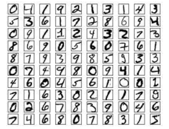
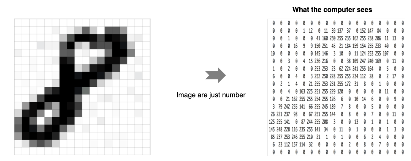
The MNIST dataset using handwritten digits is shown in the figure above. The dataset contains 60000 samples for training and 10000 samples for testing. The image is a fixed size (28x28 pixels) with values from 0 to 255.

The implementation process of the whole case is:

• Data loading
• data processing
• model building
• model training
• Model test
• Model saving

First, import the required Toolkit:

# Import the corresponding Toolkit
import numpy as np
import matplotlib.pyplot as plt
plt.rcParams['figure.figsize'] = (7,7) # Make the figures a bit bigger
import tensorflow as tf
# data set
from tensorflow.keras.datasets import mnist
# Build sequence model
from tensorflow.keras.models import Sequential
# Import required layers
from tensorflow.keras.layers import Dense, Dropout, Activation,BatchNormalization
# Import auxiliary Kit
from tensorflow.keras import utils
# Regularization
from tensorflow.keras import regularizers

Data loading

First, load the handwritten digital image

# Total categories
nb_classes = 10
# Load dataset
(X_train, y_train), (X_test, y_test) = mnist.load_data()
# Dimensions of the printout dataset
print("Initial dimension of training sample", X_train.shape)
print("Initial dimension of target value of training sample", y_train.shape)

The result is:

Initial dimension of training sample (60000, 28, 28)
Initial dimension of target value of training sample (60000,)

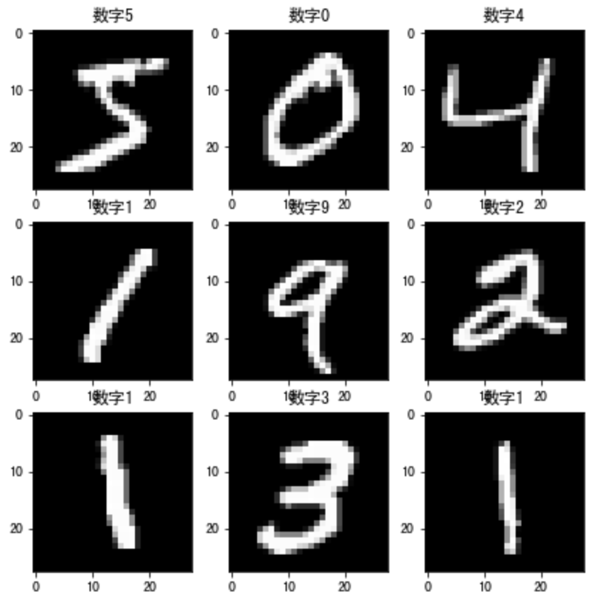
Data display:

# Data display: display the first nine data sets of the data set
for i in range(9):
    plt.subplot(3,3,i+1)
    # Displayed in grayscale without interpolation
    plt.imshow(X_train[i], cmap='gray', interpolation='none')
    # Set the title of the picture: corresponding category
    plt.title("number{}".format(y_train[i]))

The effect is as follows:

data processing

Each training sample in the neural network is a vector, so it is necessary to reshape the input to make each 28x28 image a 784 dimensional vector. In addition, the input data is normalized and adjusted from 0-255 to 0-1.

# Adjust data dimension: convert each number into a vector
X_train = X_train.reshape(60000, 784)
X_test = X_test.reshape(10000, 784)
# format conversion
X_train = X_train.astype('float32')
X_test = X_test.astype('float32')
# normalization
X_train /= 255
X_test /= 255
# Dimension adjusted results
print("Training set:", X_train.shape)
print("Test set:", X_test.shape)

Output is:

Training set: (60000, 784)
Test set: (10000, 784)

In addition, we also need to process the target value and convert it into the form of thermal coding:

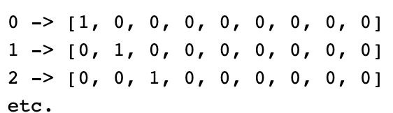
The implementation method is as follows:

# Convert the target value to hot coded form
Y_train = utils.to_categorical(y_train, nb_classes)
Y_test = utils.to_categorical(y_test, nb_classes)

model building

Here, we build a network with only three layers of full connection for processing:

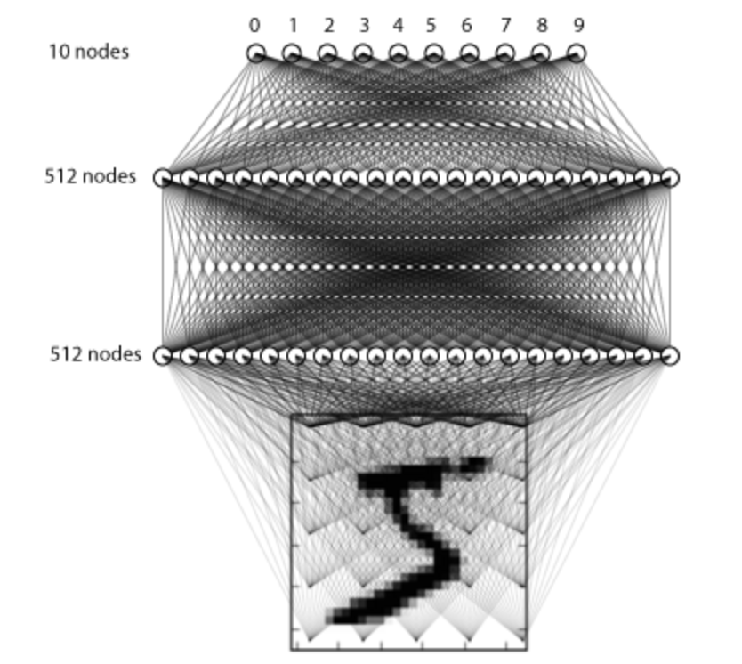
The construction method is as follows:

# Using sequence model to build model
model = Sequential()
# There are 512 neurons in the whole connection layer, and the input dimension is 784
model.add(Dense(512, input_shape=(784,)))
# The activation function uses relu
model.add(Activation('relu')) 
# Using the regularization method drouout                           
model.add(Dropout(0.2))  
# There are 512 neurons in the whole connection layer, and L2 regularization is added
model.add(Dense(512,kernel_regularizer=regularizers.l2(0.001)))
# BN layer
model.add(BatchNormalization())
# Activation function
model.add(Activation('relu'))
model.add(Dropout(0.2))
# There are 10 neurons in the whole connection layer and the output layer
model.add(Dense(10))
# softmax converts the score output by the neural network into a probability value
model.add(Activation('softmax')) 

We passed the model In summary, see the following results:

Model: "sequential_6"
_________________________________________________________________
Layer (type)                 Output Shape              Param #   
=================================================================
dense_13 (Dense)             (None, 512)               401920    
_________________________________________________________________
activation_8 (Activation)    (None, 512)               0         
_________________________________________________________________
dropout_7 (Dropout)          (None, 512)               0         
_________________________________________________________________
dense_14 (Dense)             (None, 512)               262656    
_________________________________________________________________
batch_normalization (BatchNo (None, 512)               2048      
_________________________________________________________________
activation_9 (Activation)    (None, 512)               0         
_________________________________________________________________
dropout_8 (Dropout)          (None, 512)               0         
_________________________________________________________________
dense_15 (Dense)             (None, 10)                5130      
_________________________________________________________________
activation_10 (Activation)   (None, 10)                0         
=================================================================
Total params: 671,754
Trainable params: 670,730
Non-trainable params: 1,024
_________________________________________________________________

Model compilation

Set the loss function used for model training, cross entropy loss and optimization method adam. The loss function is used to measure the difference between the predicted value and the real value, and the optimizer is used to achieve the optimization by using the loss function:

# Model compilation, indicating the loss function and optimizer, and evaluating indicators
model.compile(loss='categorical_crossentropy', optimizer='adam',metrics=['accuracy'])

model training

# batch_size is the number of samples sent into the model each time, epichs is the number of iterations of all samples, and indicates the validation data set
history = model.fit(X_train, Y_train,
          batch_size=128, epochs=4,verbose=1,
          validation_data=(X_test, Y_test))

The training process is as follows:

Epoch 1/4
469/469 [==============================] - 2s 4ms/step - loss: 0.5273 - accuracy: 0.9291 - val_loss: 0.2686 - val_accuracy: 0.9664
Epoch 2/4
469/469 [==============================] - 2s 4ms/step - loss: 0.2213 - accuracy: 0.9662 - val_loss: 0.1672 - val_accuracy: 0.9720
Epoch 3/4
469/469 [==============================] - 2s 4ms/step - loss: 0.1528 - accuracy: 0.9734 - val_loss: 0.1462 - val_accuracy: 0.9735
Epoch 4/4
469/469 [==============================] - 2s 4ms/step - loss: 0.1313 - accuracy: 0.9768 - val_loss: 0.1292 - val_accuracy: 0.9777

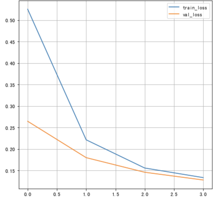
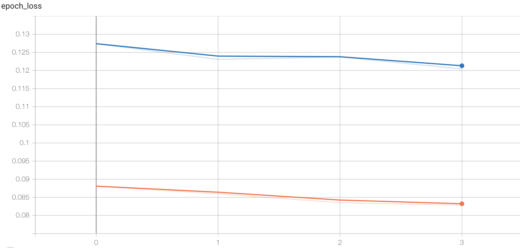
Curve the loss:

# Draw the change curve of loss function
plt.figure()
# Training set loss function transformation
plt.plot(history.history["loss"], label="train_loss")
# Verification set loss function change
plt.plot(history.history["val_loss"], label="val_loss")
plt.legend()
plt.grid()

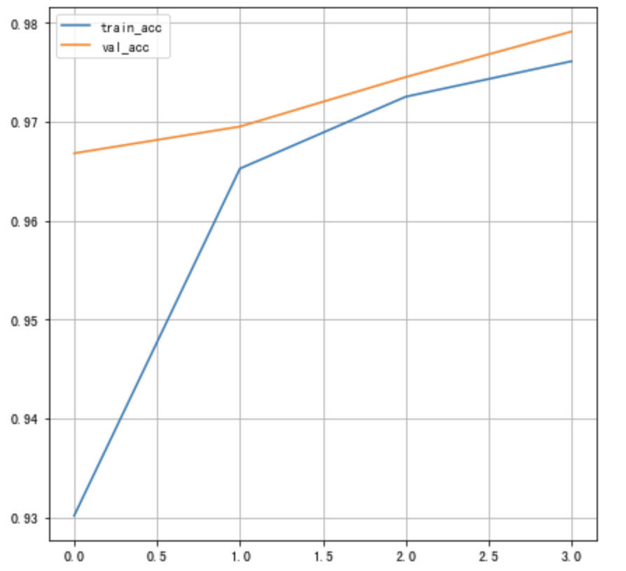
Draw the accuracy of training as a curve:

# Draw the change curve of accuracy
plt.figure()
# Training set accuracy
plt.plot(history.history["accuracy"], label="train_acc")
# Verification set accuracy
plt.plot(history.history["val_accuracy"], label="val_acc")
plt.legend()
plt.grid()

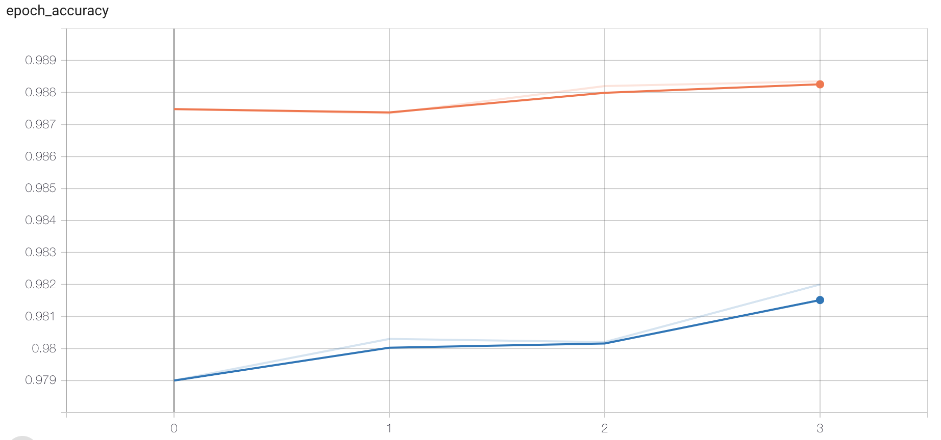
In addition, the training process can be monitored through tensorboard. At this time, we specify the callback function:

# Add tensoboard observation
tensorboard = tf.keras.callbacks.TensorBoard(log_dir='./graph', histogram_freq=1,
                                                write_graph=True,write_images=True)

During training:

# train
history = model.fit(X_train, Y_train,
          batch_size=128, epochs=4,verbose=1,callbacks=[tensorboard],
          validation_data=(X_test, Y_test))

Open the terminal:

# Specify the directory where the file exists and open the following command
tensorboard --logdir="./"

Open the specified website in the browser to view the changes of loss function and accuracy, graph structure, etc.

Model test

# Model test
score = model.evaluate(X_test, Y_test, verbose=1)
# Print results
print('Test set accuracy:', score)

result:

313/313 [==============================] - 0s 1ms/step - loss: 0.1292 - accuracy: 0.9777
Test accuracy: 0.9776999950408936

Model saving

# Save model architecture and weights in h5 file
model.save('my_model.h5')
# The weight of the loaded model and the corresponding schema include:
model = tf.keras.models.load_model('my_model.h5')

summary

• Able to use TF Keras get dataset:

load_data()

• It can construct multilayer neural network

Deny, activation function, dropout,BN layer, etc

• Be able to complete network training and evaluation

fit, callback function, evaluate, save model