Author home page( Silicon based workshop of slow fire rock sugar): Slow fire rock sugar (Wang Wenbing) blog silicon based workshop of slow fire rock sugar _csdnblog
Website of this article: https://blog.csdn.net/HiWangWenBing/article/details/120605366
catalogue
Introduction deep learning model framework
Chapter 1 business area analysis
one point one Step 1-1: business domain analysis
1.2 steps 1-2: Business Modeling
1.3 code instance preconditions
Chapter 2 definition of forward operation model
two point one Step 2-1: dataset selection
two point two Step 2-2: Data Preprocessing
2.3 step 2-3: neural network modeling
2.4 steps 2-4: neural network output
Chapter 3 definition of backward operation model
3.1 step 3-1: define the loss function
three point two Step 3-2: define the optimizer
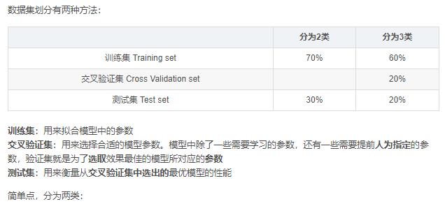
3.4 step 3-4: model validation
3.5 step 3-5: Model Visualization
4.1 step 4-1: model deployment
Introduction deep learning model framework
 https://blog.csdn.net/HiWangWenBing/article/details/120462734
Chapter 1 business area analysis
one point one Step 1-1: business domain analysis

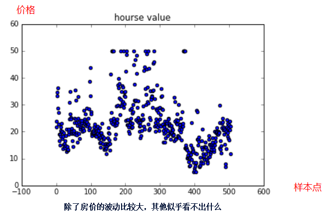
The fluctuation of house prices seems irregular, but there are 12 factors that determine house prices, and there are indeed rules to follow.
Therefore, this problem is actually a nonlinear regression problem of multivariate function:
Independent variables: 12 dimensions that determine house prices.
Dependent variable: final house price.
There are 13 influencing factors.
1.2 steps 1-2: Business Modeling
A single neuron is both an input and a single output.
Two layers of neural networks can be constructed:
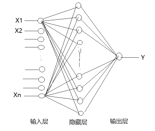
(1) Hidden layer 1:
- Number of input attributes: 13
- Number of neurons in hidden layer: 30
- Hidden layer activation function: relu
(2) Output layer:
- Number of input attributes: 30
- Number of neurons in hidden layer: 1
- Hidden layer activation function: None
1.3 code instance preconditions
#Environmental preparation
import numpy as np              # numpy array library
import math                     # Mathematical operation Library
import matplotlib.pyplot as plt # Drawing library

import torch             # torch base library
import torch.nn as nn    #  torch neural network library
import torch.nn.functional as F    #  torch neural network library
from sklearn.datasets import load_boston
from sklearn.preprocessing import MinMaxScaler
from sklearn.model_selection import train_test_split

print("Hello World")
print(torch.__version__)
print(torch.cuda.is_available())
Hello World 1.8.0 False
Chapter 2 definition of forward operation model
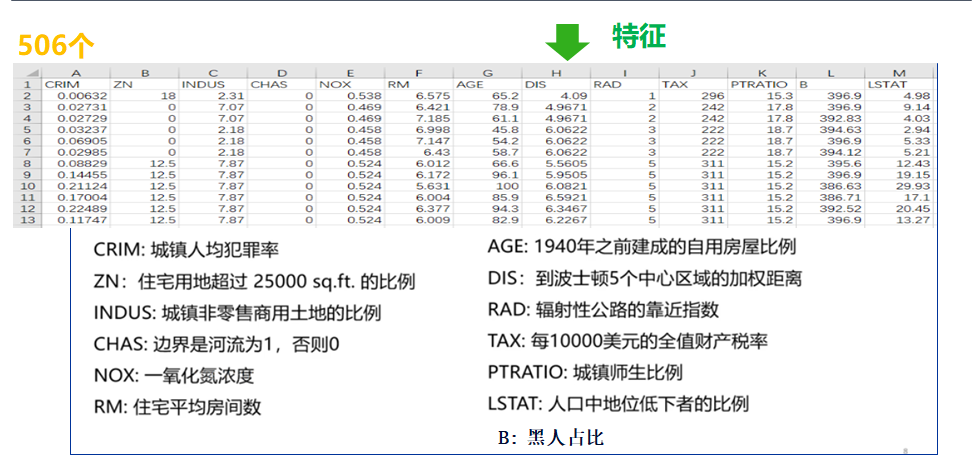
two point one Step 2-1: dataset selection
Here, the remote online download data set is adopted: data_url =“ http://lib.stat.cmu.edu/datasets/boston "
The tool for remotely downloading datasets comes from: from sklearn.datasets import load_boston
#2-1 preparing data sets
full_data = load_boston()
# Advance sample data
x_raw_data = full_data['data']
print(x_raw_data.shape)
#Extract sample label
y_raw_data = full_data['target']
print(y_raw_data.shape)
y_raw_data = y_raw_data.reshape(-1,1)
print(y_raw_data.shape)
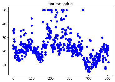
# Fluctuation range of house prices
plt.scatter(range(len(y_raw_data)), y_raw_data, color="blue")
plt.title("hourse value")(506, 13) (506,) (506, 1)
two point two Step 2-2: Data Preprocessing
# 2-2 data preprocessing
print("Data normalization preprocessing, shape unchanged, content changed")
ss = MinMaxScaler()
x_data = ss.fit_transform(x_raw_data)
y_data = y_raw_data
print(x_data.shape)
print(y_data.shape)

print("\n hold x,y from ndarray Format conversion torch format")
x_sample = torch.from_numpy(x_data).type(torch.FloatTensor)
y_sample = torch.from_numpy(y_data).type(torch.FloatTensor)
print(x_sample.shape)
print(y_sample.shape)

print("\n The data set is cut into training data set and test data set")
# 0.2 indicates the proportion of the test set
x_train,x_test, y_train, y_test = train_test_split(x_sample , y_sample, test_size=0.2)
print(x_train.shape)
print(y_train.shape)
print(x_test.shape)
print(y_test.shape)
Data normalization preprocessing, shape unchanged, content changed (506, 13) (506, 1) Convert x and y from ndarray format to torch format torch.Size([506, 13]) torch.Size([506, 1]) The data set is cut into training data set and test data set torch.Size([404, 13]) torch.Size([404, 1]) torch.Size([102, 13]) torch.Size([102, 1])
2.3 step 2-3: neural network modeling
# 2-3 define network model
class Net(torch.nn.Module):
    # Defining neural networks
    def __init__(self, n_feature, n_hidden, n_output):
        super(Net, self).__init__()
        #Define hidden layer L1
        # n_feature: enter the dimension of the attribute
        # n_hidden: number of neurons = number of output attributes
        self.hidden = torch.nn.Linear(n_feature, n_hidden)

        #Define output layer:
        # n_hidden: enter the dimension of the attribute
        # n_output: number of neurons = number of output attributes
        self.predict = torch.nn.Linear(n_hidden, n_output)

    #Define forward operation
    def forward(self, x):
        h1 = self.hidden(x)
        a1 = F.relu(h1)
        out = self.predict(a1)
        a2 = F.relu(out)
        return a2

model = Net(13,30,1)
print(model)
print(model.parameters)
print(model.parameters())
Net( (hidden): Linear(in_features=13, out_features=30, bias=True) (predict): Linear(in_features=30, out_features=1, bias=True) ) <bound method Module.parameters of Net( (hidden): Linear(in_features=13, out_features=30, bias=True) (predict): Linear(in_features=30, out_features=1, bias=True) )> <generator object Module.parameters at 0x000002922E120900>
2.4 steps 2-4: neural network output
# 2-4 define network prediction output
y_pred = model.forward(x_train)
print(y_pred.shape)
torch.Size([404, 1])
Chapter 3 definition of backward operation model
3.1 step 3-1: define the loss function
The MSE loss function used here
# 3-1 define the loss function:
# loss_fn= MSE loss
loss_fn = nn.MSELoss()

print(loss_fn)
MSELoss()
three point two Step 3-2: define the optimizer
# 3-2 defining the optimizer
Learning_rate = 0.01     #Learning rate

# optimizer = SGD: basic gradient descent method
# Parameters: indicates the list of parameters to be optimized
# lr: indicates the learning rate
optimizer = torch.optim.SGD(model.parameters(), lr = Learning_rate)
print(optimizer)
SGD (
Parameter Group 0
    dampening: 0
    lr: 0.01
    momentum: 0
    nesterov: False
    weight_decay: 0
)
3.3 step 3-3: model training
# 3-3 model training
# Define the number of iterations
epochs = 100000

loss_history = [] #loss data during training
y_pred_history =[] #Intermediate forecast results

for i in range(0, epochs):

    #(1) Forward calculation
    y_pred = model(x_train)

    #(2) Calculate loss
    loss = loss_fn(y_pred, y_train)

    #(3) Reverse derivation
    loss.backward()

    #(4) Reverse iteration
    optimizer.step()

    #(5) Reset the gradient of the optimizer
    optimizer.zero_grad()

    # Record training data
    loss_history.append(loss.item())
    y_pred_history.append(y_pred.data)

    if(i % 10000 == 0):
        print('epoch {}  loss {:.4f}'.format(i, loss.item()))

print("\n Iteration completion")
print("final loss =", loss.item())
print(len(loss_history))
print(len(y_pred_history))
epoch 0 loss 573.5384 epoch 10000 loss 5.3641 epoch 20000 loss 3.6727 epoch 30000 loss 3.0867 epoch 40000 loss 2.8373 epoch 50000 loss 2.2653 epoch 60000 loss 2.3308 epoch 70000 loss 2.1467 epoch 80000 loss 1.9769 epoch 90000 loss 1.7896 Iteration completion final loss = 1.9121897220611572 100000 100000
3.4 step 3-4: model validation
(1) Validation on training set
# Use the training set data to check the training effect
y_train_pred = model.forward(x_train)

loss_train = torch.mean((y_train_pred - y_train)**2)
print("loss for train:", loss_train.data)

plt.scatter(range(len(y_train)), y_train.data, color="blue")
plt.scatter(range(len(y_train_pred)), y_train_pred.data, color="red")
plt.title("hourse value")
loss for train: tensor(1.8895)
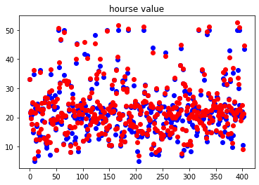
Validation results on the training set:
- Average loss: 1.8895
- The predicted points are close to the actual sample points.
(2) Validation on test set
# Use the test set data to verify the test effect
y_test_pred = model.forward(x_test)

loss_test = torch.mean((y_test_pred - y_test)**2)
print("loss for test:", loss_test.data)

plt.scatter(range(len(y_test)), y_test.data, color="blue")
plt.scatter(range(len(y_test_pred)), y_test_pred.data, color="red")
plt.title("hourse value")
loss for test: tensor(38.7100)
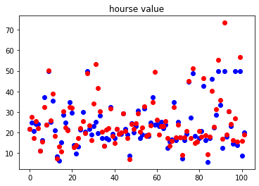
Validation results on the training set:
- The average loss is 38.7100, which is multiplied by the training set
- The predicted points deviate greatly from the actual sample points
- The loss of the model on the training set is much better than that on the test set, and the generalization ability of the model is poor.
3.5 step 3-5: Model Visualization
(1) Forward data
(2) Backward loss iterative process
Display all loss data:
#Display historical data of loss
plt.plot(loss_history, "r+")
plt.title("loss value")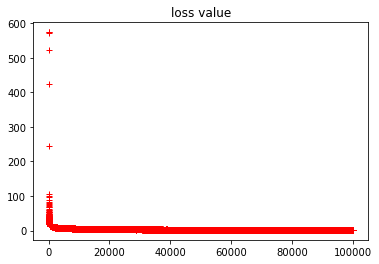
Ignoring the data of early rapid convergence, it shows the local convergence of loss
#Display historical data of loss
plt.plot(loss_history[1000::], "r+")
plt.title("loss value") 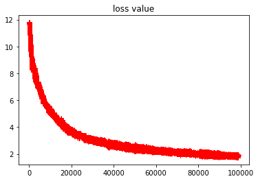
(3) Iterative process of forward prediction function
Chapter 4 model deployment
4.1 step 4-1: model deployment
NA
Author home page( Silicon based workshop of slow fire rock sugar): Slow fire rock sugar (Wang Wenbing) blog silicon based workshop of slow fire rock sugar _csdnblog
Website of this article: https://blog.csdn.net/HiWangWenBing/article/details/120605366