Article content

1, Selective sorting method
Selective sorting is to repeatedly take out the smallest (or largest) data from the unordered sequence and store it at the beginning of the sequence, and then continue to find the smallest (or largest) data from the unordered elements and store it at the end of the sorted sequence. The final result is the sorted sequence. The final results of the selection sorting method have two forms, namely, increasing sequence and decreasing sequence. The specific sorting processes of the two result forms are described below.
- The result is incremental sorting: first, take the minimum value in the unordered sequence and exchange with the first position of the sequence; Then take the minimum value from the unordered sequence and exchange it with the second position of the sequence. This is repeated until the data in the sorting sequence is sorted from small to large.
- The result is descending sorting: first, take the maximum value in the unordered sequence and exchange with the first position of the sequence; Then take the maximum value from the unordered sequence and exchange it with the second position of the sequence. This is repeated until the data in the sorting sequence is sorted from large to small.
Next, a set of data is used to explain the selection sorting method in detail. For example, there is a set of data: 56, 18, 49, 84, 72, as shown in the figure below:

Sort in ascending order as follows:
Step 1: find the minimum value 18 in the sequence shown and exchange it with the first element 56 in the sequence, as shown in the following figure:

Step 2: starting from the second value, find the minimum value 49 in this series (excluding the first value), and then exchange with the second value 56, as shown in the following figure:
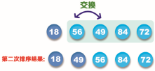
Step 3: starting from the third value, find the minimum value 56 in this sequence (excluding the first and second values). Since it is originally in the third position, it does not need to be exchanged.

Step 4: starting from the fourth value, find the minimum value 72 in this series (excluding the first, second and third values), and then exchange with the fourth value 84, as shown in the following figure:

Step 5: the sequence is sorted in ascending order, and the result is shown in the following figure:

[example 1] use the selective sorting method for incremental sorting. Use the selective sorting method to sort the list: 56, 18, 49, 84, 72 in increments. The specific codes are as follows:
def choose(data, data_len):  # Customize a selection sort method function
    for m in range(data_len - 1):  # Traverse new data
        for n in range(m + 1, data_len):
            if data[n] < data[m]:  # If the data is smaller than the original data
                data[m], data[n] = data[n], data[m]  # Need to swap locations
        print('The first %d The result after sorting is' % (m + 1), end='')  # Tips
        for n in range(data_len):  # Traverse the results of each sort
            print('%3d' % data[n], end='')  # Output results
        print()  # Output blank line


num_list = [56, 18, 49, 84, 72]  # Create series and initialize
length = len(num_list)
print("The original data are:")  # Tips
for i in range(length):  # Traverse the original data
    print('%3d' % num_list[i], end='')  # Output results
print('\n---------------------------')  # Output delimiter
choose(num_list, length)  # Call the select sort method function
print('\n---------------------------')  # Output delimiter
print("The sorted data is:")  # Tips
for j in range(length):  # Traverse the data of the sorted new sequence
    print('%3d' % num_list[j], end='')  # Output results
print('')  # Output blank line
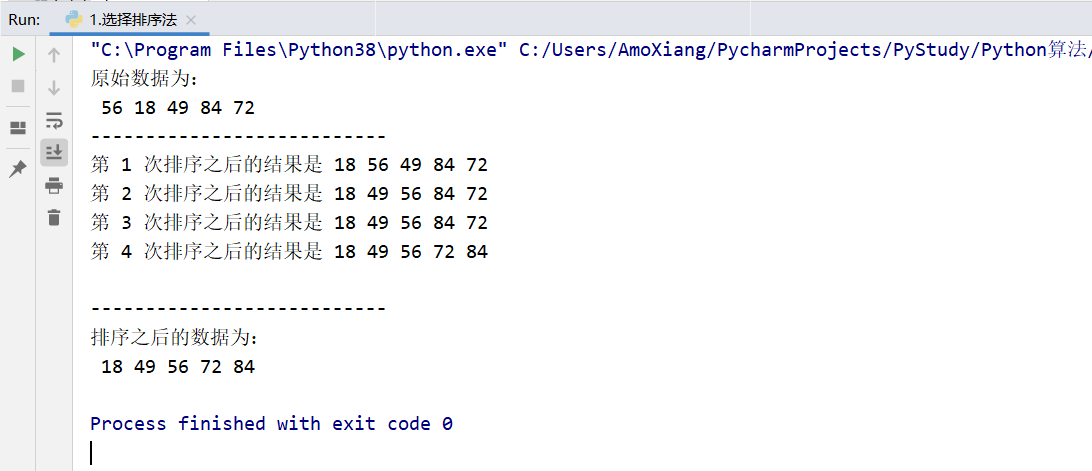
The running results of the program are shown in the figure below:
2, Bubble sorting
Bubble sorting method is a sorting method created by observing the changes of bubbles in the water. Its basic principle is to start from the first data and compare the size of adjacent data. If the size order is wrong, adjust it and then compare it with the next data, just like when bubbles gradually rise from the bottom to the surface of the water. After such continuous exchange, the correct location of the last data can be found. Then exchange step by step until the sorting of all data is completed.
The final result of bubble sorting method also has two forms: increasing sequence and decreasing sequence. Next, a set of data is used to explain the basic principle of bubble sorting method in detail.
For example, there is a set of data: 56, 20, 84, 66, 13, as shown in the following figure:

Sort in ascending order as follows:
Step 1: first, compare the data 56 of the first position with the data 20 of the second position. Because 20 is less than 56, exchange it; Then, the data 56 of the second position is compared with the data 84 of the third position. Because 56 is less than 84, there is no need to exchange; Then compare the data 84 of the third position with the data 66 of the fourth position. Because 66 is less than 84, it is exchanged; Finally, the data 84 of the fourth position is compared with the data 13 of the fifth position. Because 84 is greater than 13, it is exchanged. This completes the first sorting. The sorting process is shown in the following figure:
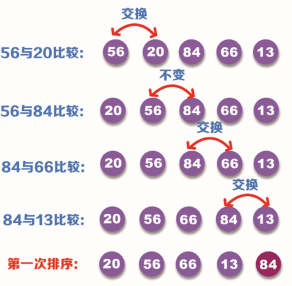
Step 2: after the first sorting, the maximum value 84 has been placed in the corresponding position, so it can be compared to 13 in the second sorting.
The second sorting still starts from the first position, that is, compare the size of data 20 and 56. Because 20 is less than 56, there is no need to exchange; Then compare the sizes of data 56 and 66. Because 56 is less than 66, there is no need to exchange; Finally, compare the size of data 66 and 13. Because 66 is greater than 13, it needs to be exchanged. This completes the second sorting. The sorting process is shown in the following figure:
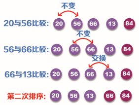
Step 3: after the second sorting, the maximum value 66 of the remaining sequence (except 84) has been placed in the corresponding position, so it can be compared to 13 in the third sorting.
The third sorting still starts from the first position, that is, compare the size of data 20 and 56. Because 20 is less than 56, there is no need to exchange positions; Then compare the sizes of data 56 and 13. Because 56 is greater than 13, it is necessary to exchange positions. This completes the third sorting. The sorting process is shown in the following figure:
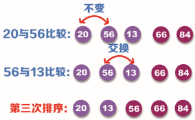
Step 4: after the third sorting, the number series 84, 66 and 56 have been placed in the corresponding position, so it can be compared to 13 in the fourth sorting.
The fourth sorting still starts from the first position. Compare the size of data 20 and 13. Because 20 is greater than 13, it is necessary to exchange positions. This completes the fourth sorting. The sorting process is shown in the following figure:
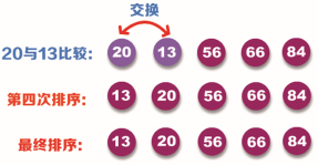
At this point, the sorting is completed.
[example 2] the bubble sorting method is used for incremental sorting. Use bubble sorting method to sort the list: 56, 20, 84, 66, 13 in increments. The specific codes are as follows:
def bubble(data, data_len):  # Customize a bubble sorting function
    traversal_times = data_len - 1
    for m in range(traversal_times, 0, -1):  # Traversal sorting times
        for n in range(m):  # Traverse new data
            if data[n + 1] < data[n]:  # If the data is smaller than the original data
                data[n], data[n + 1] = data[n + 1], data[n]  # Need to swap locations
        print('The first %d The result after sorting is' % (data_len - m), end='')  # Tips
        for n in range(data_len):  # Traverse the results of each sort
            print('%3d' % data[n], end='')  # Output results
        print()  # Output blank line


num_list = [56, 20, 84, 66, 13]  # Create series and initialize
length = len(num_list)
print("The original data are:")  # Tips
for i in range(length):  # Traverse the original data
    print('%3d' % num_list[i], end='')  # Output results
print('\n---------------------------')  # Output delimiter
bubble(num_list, length)  # Call bubble sort function
print('---------------------------')  # Output delimiter
print("The sorted data is:")  # Tips
for i in range(length):  # Traverse the data of the sorted new sequence
    print('%3d' % num_list[i], end='')  # Output results
print('')  # Output blank line
The running results of the program are shown in the figure below:

From the running results shown in the figure above, the sorting steps are completely consistent with the bubble sorting method described above.
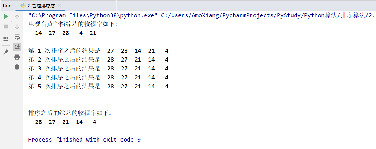
[exercise 1] ranking of variety ratings of various TV stations in the golden file. Now, each TV station will have its own variety show in the prime time slot every Friday. The ratings of the prime time slot variety show in a certain week are as follows: 14, 27, 28, 04, 21 (omitting its%). The ratings are sorted from high to low by bubble sorting method. The program operation results are shown in the following figure:
3, Direct insertion sorting
Direct insertion sorting method is to compare the data in the sequence with the sorted data one by one. For example, if you insert the third data into the two data arranged in order, you need to compare it with the two data arranged, and put the data in the appropriate position through the comparison results. That is, when the third data is inserted into the sequence, the three data are already in order. Then insert the fourth data, and so on, until the sorting is completed.
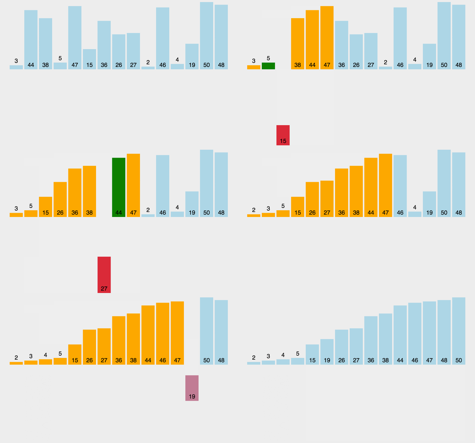
The final result of direct insertion sorting method also has two forms: increasing sequence and decreasing sequence. Next, a set of numerical sequences is used to demonstrate the sorting of direct insertion sorting method. For example, there is a set of numbers: 58, 29, 86, 69, 10, as shown in the figure below:
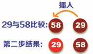
Step 3: compare the data 86 in the third position with 29 and 58. Because 86 is greater than 29 and 58, put 86 directly in the third position, as shown in the following figure:

Step 4: compare the data 69 in the fourth position with 29, 58 and 86. Because 69 is greater than 29 and 58 and 69 is less than 86, insert 69 directly into the position in front of 86 and move 86 back one bit, as shown in the following figure:

Step 5: compare the data 10 in the fifth position with 29, 58, 69 and 86 respectively. Because 10 is less than 29, 58, 69 and 86, insert 10 directly into the position in front of 29 and move 29, 58, 69 and 86 backward one bit in turn, as shown in the following figure:

The final sorting result of direct insertion sorting is shown in the following figure:

At this point, the sorting is completed.
[example 3] the direct insertion sorting method is used for incremental sorting. Use the direct insertion sort method to sort the list: 58, 29, 86, 69, 10 incrementally. The specific codes are as follows:
def insert(data):  # Customize an insertion sort method function
    for i in range(5):  # Traverse new data
        temp = data[i]  # temp is used to temporarily store data
        j = i - 1
        # Cyclic sorting: the judgment condition is that the subscript value of the data must be greater than or equal to 0 and the temporary data is less than the original data
        while j >= 0 and temp < data[j]:
            data[j + 1] = data[j]  # Move all elements back one bit
            j -= 1  # Subscript minus 1
        data[j + 1] = temp  # The smallest data is inserted into the first position
        print('The first %d The result after sorting is' % (i + 1), end='')  # Tips
        for j in range(5):  # Traverse the results of each sort
            print('%3d' % data[j], end='')  # Output results
        print()  # Output blank line


data = [58, 29, 86, 69, 10]  # Create series and initialize
print("The original data are:")  # Tips
for i in range(5):  # Traverse the original data
    print('%3d' % data[i], end='')  # Output results
print('\n---------------------------')  # Output delimiter
insert(data)  # Call the direct insertion sort method function
print('\n---------------------------')  # Output delimiter
print("The sorted data is:")  # Tips
for i in range(5):  # Traverse the data of the sorted new sequence
    print('%3d' % data[i], end='')  # Output results
print('')  # Output blank line
The running results of the program are shown in the figure below:
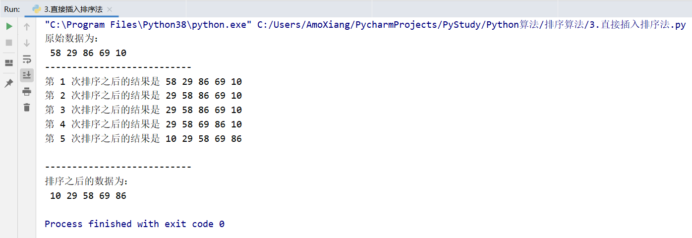
From the results shown in the figure above, the results are completely consistent with the steps of direct insertion sorting method introduced above.
[exercise 2] output the ranking of rope skipping results. Body is the capital of revolution, and physical exercise is a very important thing. Therefore, the content of the middle school entrance examination has been added to the physical examination, and rope skipping is one of the examination contents. For example, the number of rope skipping of five candidates in the middle school entrance examination of a school is as follows: 1551381185149163. The direct insertion method is used to rank the five candidates from high to low. The specific code is as follows:
def insert(data):  # Customize an insertion sort method function
    for i in range(5):  # Traverse new data
        temp = data[i]  # temp is used to temporarily store data
        j = i - 1
        # Cyclic sorting: the judgment condition is that the subscript value of the data must be greater than or equal to 0 and the temporary data is greater than the original data
        while j >= 0 and temp > data[j]:
            data[j + 1] = data[j]  # Move all elements back one bit
            j -= 1  # Subscript minus 1
        data[j + 1] = temp  # The smallest data is inserted into the first position
        print('The first %d The result after sorting is' % (i + 1), end='')  # Tips
        for j in range(5):  # Traverse the results of each sort
            print('%6d' % data[j], end='')  # Output results
        print()  # Output blank line


data = [155, 138, 185, 149, 163]  # Create series and initialize
print("The number of rope skipping for the five candidates is as follows:")  # Tips
for i in range(5):  # Traverse the original data
    print('%6d' % data[i], end='')  # Output results
print('\n---------------------------')  # Output delimiter
insert(data)  # Call the direct insertion sort method function
print('\n---------------------------')  # Output delimiter
print("The number of rope skipping after ranking from high to low is as follows:")  # Tips
for i in range(5):  # Traverse the data of the sorted new sequence
    print('%6d' % data[i], end='')  # Output results
print('')
The running results of the program are shown in the figure below:
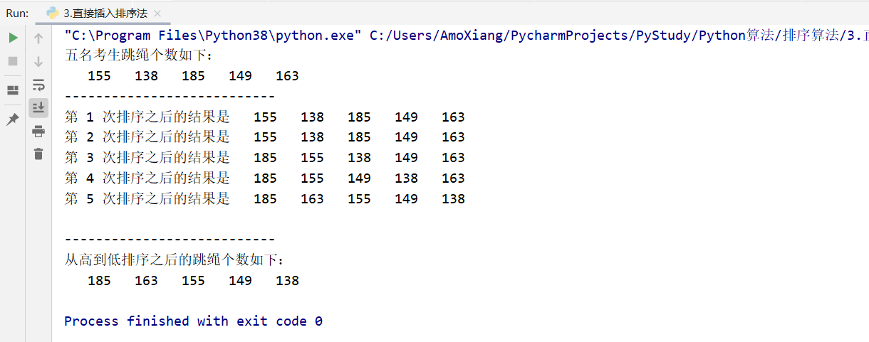
4, Merge sort method
Merge sort method is to combine two or more sorted series into a large and sorted series by merging. First, divide the unordered sequence into several small parts. The rule of dividing several parts is to divide the length of each section by 2 (half to half) until it cannot be divided again, then sort the divided sequence, and finally gradually merge it into a sorted large sequence, as shown in the figure below:
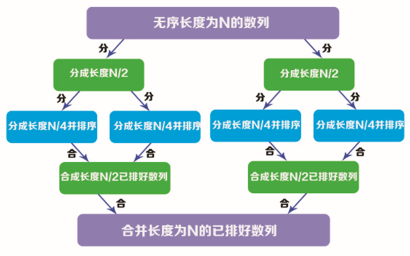
The final result of merge sorting method also has two forms, namely, increasing sequence and decreasing sequence. Next, a group of data is used to demonstrate the sorting principle of merge sorting method. For example, there is a set of data: 33, 10, 49, 78, 57, 96, 66, 21, as shown in the figure below:

Sort by increment, as follows:
Step 1: divide the original sequence into two to get two sequences, namely sequence 1 and sequence 2. Sequence 1 is 33, 10, 49 and 78; Sequence 2 is 57, 96, 66 and 21, as shown in the figure below:

Step 2: divide the sequence 1 and sequence 2 shown in the above figure into two to obtain sequence a, sequence b, Sequence c and sequence d. At this time, each series contains two data, and the two data in each series are sorted, as shown in the following figure:

Step 3: merge the sorted sequence elements in the above figure, and merge sequence a and sequence B into sequence a; Merge Sequence c and sequence d into sequence B. Then sort the data elements in sequence a and sequence B, as shown in the following figure:

Step 4: merge sequence A and sequence B in the above figure into one sequence, and sort the internal data. The final sorting result is shown in the figure below:

At this point, the sorting is completed.
[example 4] use the merge sort method to sort incrementally. Use the merge sort method to sort the list: 33, 10, 49, 78, 57, 96, 66, 21. The specific codes are as follows:
def merge_sort(data):  # Custom merge sort function
    if len(data) <= 1:  # Judge whether the list element is less than or equal to 1
        return data  # When there is only one list element, it is returned directly
    mid = len(data) // 2 # separation length calculation, the length of the whole data is rounded by dividing by 2
    left = data[:mid]  # Left half data
    right = data[mid:]  # Right half data
    left = merge_sort(left)  # Call merge_ The sort() function continues to separate and sort the left half
    right = merge_sort(right)  # Call merge_ The sort() function continues to separate and sort the right half
    # Sort recursively
    result = []  # Used to store the result value
    while left and right:  # For circular merging, the judgment condition is: whether the left subscript and right subscript are true
        if left[0] <= right[0]:  # Judge that the number on the left is less than the number on the right
            result.append(left.pop(0))  # The result increases the value of left[0]
        else:
            result.append(right.pop(0))  # The result increases the value of right[0]
    if left:  # If the value of left is true
        result += left  # The result shows the data on the left
    if right:  # If the value of right is true
        result += right  # The result shows the data on the right
    return result  # Returns the sorted result


data = [33, 10, 49, 78, 57, 96, 66, 21]  # Create series and initialize
print("The original data are:", data)  # Output raw data
print('------------------------------------------------------')  # Output delimiter
print("The sorted data is:", merge_sort(data))  # Call the function to output the sorted data
print('------------------------------------------------------')  # Output delimiter
The running results of the program are shown in the figure below:

[exercise 3] ranking of mobile phone sales of "double eleven" brand. "Double 11" is an annual shopping carnival, with countless businesses participating. Of course, brand mobile phones are also one of the hot sales goods of "double 11". Suppose that the sales volume of mobile phones of five brands (10000 units) are 27503429163240193698 respectively. The consolidated sorting method is used to sort the sales volume from high to low. The specific code is as follows:
def merge_sort(data):  # Custom merge sort function
    if len(data) <= 1:  # Judge whether the list element is less than or equal to 1
        return data  # When there is only one list element, it is returned directly
    mid = len(data) // 2 # separation length calculation, the length of the whole data is rounded by dividing by 2
    left = data[:mid]  # Left half data
    right = data[mid:]  # Right half data
    left = merge_sort(left)  # Call merge_ The sort() function continues to separate and sort the left half
    right = merge_sort(right)  # Call merge_ The sort() function continues to separate and sort the right half
    # Sort recursively
    result = []  # Used to store the result value
    while left and right:  # For circular merging, the judgment condition is: whether the left subscript and right subscript are true
        if left[0] >= right[0]:  # Judge that the number on the left is greater than the number on the right
            result.append(left.pop(0))  # The result increases the value of left[0]
        else:
            result.append(right.pop(0))  # The result increases the value of right[0]
    if left:  # If the value of left is true
        result += left  # The result shows the data on the left
    if right:  # If the value of right is true
        result += right  # The result shows the data on the right
    return result  # Returns the sorted result


data = [2750, 3429, 1632, 4019, 3698]  # Create series and initialize
print("The sales volume of five major brands of mobile phones is as follows:", data)  # Output raw data
print('================================')  # Output delimiter
print("The sales volume after ranking from high to low is as follows:", merge_sort(data))  # Call the function to output the sorted data
print('================================')  # Output delimiter
The running results of the program are shown in the figure below:

5, Hill ranking method
Hill sort method is a kind of insertion sort method, which is a more advanced improved version of direct insertion sort algorithm. Hill sorting method can reduce the number of data movement in insertion sorting method and speed up the sorting, so it is called reduced incremental sorting. The principle of hill sorting method is to divide the original data into several groups of data with specific intervals, and then use the insertion sorting method to sort each group of data. After sorting, reduce the interval distance, and then repeat the insertion sorting method to sort each group of data until all data are sorted. The final result of Hill ranking method has two forms: increasing sequence and decreasing sequence. Next, a set of data is used to demonstrate the sorting principle of hill sorting method.
For example, a set of original data: 60, 82, 17, 35, 52, 73, 54, 9, as shown in the figure below:

Sort by increment, as follows:
Step 1: as can be seen from the above figure, there are 8 data in the original value. Set the interval bits to 8 / 2 = 4, that is, the original value is divided into four groups of series: Series 1 (60, 52), series 2 (82, 73), series 3 (17, 54) and series 4 (35, 9), as shown in the following figure. Sort the data in each sequence, and exchange the data with wrong position according to the principle of small on the left and large on the right, that is, sequence 1 (52, 60), sequence 2 (73, 82), sequence 3 (17, 54) and sequence 4 (9, 35).

Note: the number of interval digits does not necessarily have to be divided by 2, which can be determined according to your own needs.
Step 2: insert and place the sequence sorted in step 1 to get the first sorting result, as shown in the following figure:

Step 3: then reduce the interval [(8 / 2) / 2 = 2], that is, the original sequence is divided into two groups: sequence 1 (52, 17, 60, 54) and sequence 2 (82, 35, 73, 9), as shown in the figure below, and then sort the data in each sequence in the figure above, and exchange the data with wrong position in the order from small to large, That is, sequence 1 (17, 52, 54, 60) and sequence 2 (9, 35, 73, 82).

Step 4: insert and place the sequence sorted in step 3 to get the second sorting result, as shown in the following figure:

Step 5: take the interval number with [((8 / 2) / 2)] 2 = 1, sort each element in the sequence after the second sorting (as shown in the above figure), and the final result is shown in the following figure:

At this point, the sorting is completed.
[example 5] Hill sorting method is used for incremental sorting. Use Hill sort to sort the list: 60, 82, 17, 35, 52, 73, 54, 9 incrementally. The specific codes are as follows:
def hill(data):  # Custom Hill sort function
    n = len(data)  # Get data length
    step = n // 2 # change the step size from large to small. The last step must be 1 to obtain the offset value of gap
    while step >= 1:  # As long as gap is within our reasonable range, we will keep grouping
        # Divide the data into two parts according to the step size, traverse all the subsequent data from the position of the step size, and specify the value range of the j subscript
        for j in range(step, n):
            while j - step >= 0:  # Compare the data of gap with the current position -
                if data[j] < data[j - step]:  # Replace the size elements in the group
                    data[j], data[j - step] = data[j - step], data[j]
                    j -= step  # Update the subscript value of the migrated element to the latest value
                else:  # Otherwise, do not replace
                    break
        step //=2 # every time the insertion sorting in the group is completed, the gap is subdivided / 2


data = [60, 82, 17, 35, 52, 73, 54, 9]  # Define list and initialize
print("raw data:")
print(data)  # Output original data
print("---------------------------------")
hill(data)  # Call custom sort function
print("Sorted data:")
print(data)  # Output sorted data
print("---------------------------------")
The running results of the program are shown in the figure below:

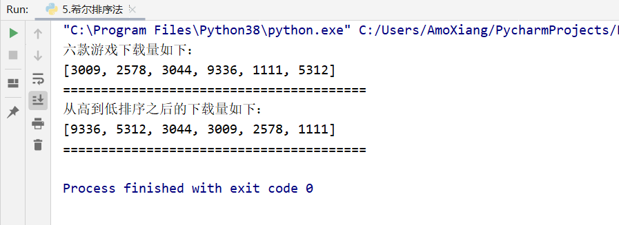
[exercise 4] ranking of popular game downloads. Games are a way for many people to spend their time. There are also various games in the software installation store of mobile phones. Suppose there are six games, and their downloads (in 10000 times) are 30092578304493361115312 respectively. Hill ranking method is used to rank the downloads from high to low. The specific codes are as follows:
def hill(data):  # Custom Hill sort function
    n = len(data)  # Get data length
    step = n // 2 # change the step size from large to small. The last step must be 1 to obtain the offset value of gap
    while step >= 1:  # As long as gap is within our reasonable range, we will keep grouping
        # Divide the data into two parts according to the step size, traverse all the subsequent data from the position of the step size, and specify the value range of the j subscript
        for j in range(step, n):
            while j - step >= 0:  # Take the data of the current location and compare it with the data of the current location gap location
                if data[j] > data[j - step]:  # Replace the size elements in the group
                    data[j], data[j - step] = data[j - step], data[j]
                    j -= step  # Update the subscript value of the migrated element to the latest value
                else:  # Otherwise, do not replace
                    break
        step //=2 # every time the insertion sorting in the group is completed, the gap is subdivided / 2


data = [3009, 2578, 3044, 9336, 1111, 5312]  # Define list and initialize
print("The downloads of the six games are as follows:")
print(data)  # Output original data
print("========================================")
hill(data)  # Call custom sort function
print("The number of downloads after ranking from high to low is as follows:")
print(data)  # After sorting data
print("========================================")
The running results of the program are shown in the figure below:
6, Quick sorting method
Quick sorting method, also known as split exchange method, is an improvement of bubble sorting method. Its basic idea is: first find a virtual intermediate value in the data, and divide all the data to be sorted into two parts according to this intermediate value. Among them, the data less than the middle value is placed on the left and the data greater than the middle value is placed on the right. The data on the left and right sides are processed in the same way until sorting is completed. The operation steps are as follows:
Suppose there are n items of data, and the data values are represented by K1, K2,..., Kn.
- First, assume a virtual intermediate value K in the data (generally take the number at the first position for convenience).
- Find the data ki from left to right so that ki > k, and the number of positions of Ki is recorded as i.
- Find the data Kj from right to left so that Kj < K, and the number of positions of Kj is recorded as j.
- If I < J, the data Ki is exchanged with Kj, and return to steps 2 and 3.
- If i ≥ j, the data K and Kj are exchanged and divided into left and right parts with j as the reference point, and then steps 1 to 5 are carried out for the left and right parts until the left half data is equal to the right half data.
The final result of quick sorting method also has two forms: increasing sequence and decreasing sequence. Next, a set of data is used to demonstrate the sorting principle of quick sorting method. For example, there is a set of data: 6, 1, 2, 7, 9, 3, 4, 5, 10, 8, as shown in the figure below:

Sort by increment, as follows:
Step 1: take the first number 6 of the original value as the virtual intermediate value, that is, K=6; Then, find the number whose value is greater than 6 from left to right, that is, the value 7, and the position is I, that is, i=4; Then look up the number with value less than 6 from right to left, i.e. value 5, and the position is j, i.e. j=8, as shown in the following figure:

Step 2: i < J, so exchange the positions of Ki (value 7) and Kj (value 5) to complete the first sorting result. Then, find the number whose value is greater than 6 from left to right, that is, the value 9, and the position is i, that is, i=5; Then find the number with value less than 6 from right to left, that is, the value 4, and the position is j, that is, j=7, as shown in the following figure:

Step 3: I < J, so exchange the positions of Ki (value 9) and Kj (value 4) to complete the second sorting. Then, find the number whose value is greater than 6 from left to right, that is, the value 9, and the position is I, that is, i=7; Then look up the number with value less than 6 from right to left, i.e. value 3. The position is j, i.e. j=6, as shown in the following figure:

Step 4: I > J, so exchange the positions of the virtual intermediate values K (value 6) and Kj (value 3) to complete the third sorting. At this time, it is found that the left half of 6 is less than 6 and the right half is more than 6. The virtual intermediate value 6 becomes the real intermediate value, as shown in the following figure:

Step 5: sort the left half data of the middle value 6. The middle value and the right half data can be ignored temporarily. Take the virtual middle value K=3 on the left half, and find the value greater than 3 from left to right, that is, the value 5, and the position is i, that is, i=4; Then find the value less than 3 from right to left, that is, the value 2, and the position is j, that is, j=3. As shown in the figure below:

Step 6: I > J, so you need to exchange the values of K (value 3) and Kj (value 2), as shown in the figure below. At this point, the virtual intermediate value becomes the real intermediate value. Those less than 3 are on the left half of the middle value 3, and those greater than 3 are on the right half of the middle value 3.

Step 7: next, sort the left and right sides with the middle value of 3. After sorting, the final sorting result is shown in the following figure:

Step 8: at this time, the left half of the whole set of data has been sorted. Next, sort the right half. This time, ignore the sorted left half and the middle value 6. Take the number of the first position on the right half as the virtual intermediate value K (value 9), and then find the value greater than 9 from left to right, that is, value 10, and the position is i, that is, i=9; Then find the value less than 9 from right to left, that is, the value 8, and the position is j, that is, j=10. As shown in the figure below:

Step 9: i < J, so exchange the positions of Ki (value 10) and Kj (value 8). Then, find the value greater than 9 from left to right, that is, the value is 10, and the position is i, that is, i=10; Then find the value less than 9 from right to left, that is, the value 8, and the position is j, that is, j=9. As shown in the figure below:

Step 10: I > J, so exchange the values of Kj (value 8) and virtual intermediate value (value 9). At this time, the virtual intermediate value becomes the real intermediate value, as shown in the following figure:

Step 11: sort the left and right sides with the middle value of 9, and finally sort the right half, as shown in the following figure:

Combining the left half sorting and the right half sorting, the final result is shown in the figure below:

This completes the sorting.
[example 6] use the quick sort method for incremental sorting. Use the quick sort method to sort the list: 6, 1, 2, 7, 9, 3, 4, 5, 10, 8 incrementally. The specific codes are as follows:
def quick(data, start, end):  # Define quicksort function
    if start > end:  # If the start value is greater than the end value
        return  # Exit the program directly
    i, j = start, end
    result = data[start]  # Take virtual intermediate value
    while True:  # loop
        while j > i and data[j] >= result:  # Look from right to left. If the number found is smaller than the virtual intermediate value, stop the cycle
            j = j - 1  # Find from right to left, position - 1 each time
        while i < j and data[i] <= result:  # Look from left to right. If the number found is greater than the virtual intermediate value, stop the cycle
            i += 1  # Find the position from left to right and + 1 each time
        if i < j:  # Both i and j stop, find the corresponding position and judge i < J
            data[i], data[j] = data[j], data[i]  # Exchange the values corresponding to positions i and j
        elif i >= j:  # Judgment I > = J
            # Exchange the virtual intermediate value and the number at the j position. At this time, the virtual intermediate value becomes the real intermediate value
            data[start], data[j] = data[j], data[start]
            break  # The first sorting is completed, and the left and right sides are divided by the middle value
    quick(data, start, i - 1)  # Call the quick sort function, and then quickly sort the left half of the data
    quick(data, i + 1, end)  # Call the quick sort function, and then quickly sort the right half of the data


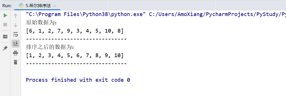
data = [6, 1, 2, 7, 9, 3, 4, 5, 10, 8]  # Define list and initialize
print("The original data are:")
print(data)  # Output raw data
print("--------------------------------")
quick(data, 0, (len(data) - 1))  # Call quick sort. The data starts at position 0 and ends at data length - 1
print("The sorted data is:")
print(data)  # Output sorted data
print("--------------------------------")
The program running results are shown in the figure:
[exercise 4] ranking of years of employment. For example, the entry years of six employees in a company are: 1, 3, 15, 20, 5 and 4. Use the quick sort method to sort the entry years of these employees from high to low. The specific codes are as follows:
def quick(data, start, end):  # Define quicksort function
    if start > end:  # If the start value is greater than the end value
        return  # Exit the program directly
    i, j = start, end
    result = data[start]  # Take virtual intermediate value
    while True:  # loop
        while j > i and data[j] <= result:  # Look from right to left. If the number found is large, the cycle will stop
            j = j - 1  # Find from right to left, position - 1 each time
        while i < j and data[i] >= result:  # Find the small value from the left to the right
            i += 1  # Find the position from left to right and + 1 each time
        if i < j:  # Both i and j stop, find the corresponding position and judge i < J
            data[i], data[j] = data[j], data[i]  # Exchange the values corresponding to positions i and j
        elif i >= j:  # Judgment I > = J
            # Exchange the virtual intermediate value and the number at the j position. At this time, the virtual intermediate value becomes the real intermediate value
            data[start], data[j] = data[j], data[start]
            break  # The first sorting is completed, and the left and right sides are divided by the middle value
    quick(data, start, i - 1)  # Call the quick sort function, and then quickly sort the left half of the data
    quick(data, i + 1, end)  # Call the quick sort function, and then quickly sort the right half of the data


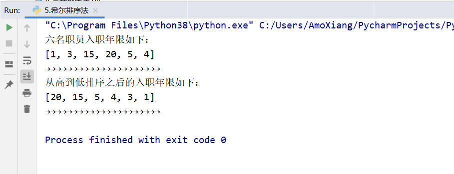
data = [1, 3, 15, 20, 5, 4]  # Define list and initialize
print("The entry years of the six employees are as follows:")
print(data)  # Output raw data
print("→→→→→→→→→→→→→→→→→→→→→")
quick(data, 0, (len(data) - 1))  # Call quick sort. The data starts at position 0 and ends at data length - 1
print("The entry years after ranking from high to low are as follows:")
print(data)  # Output sorted data
print("→→→→→→→→→→→→→→→→→→→→→")
The program running results are shown in the figure:
7, Heap sorting method
Tree structure is a structure with branches and hierarchical relationships between element nodes, which is similar to the tree in nature. In life, there are many relationships in tree structure, such as the family relationship shown in the figure below,

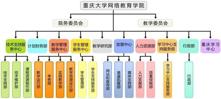
Also, the organization chart of the school of education of Chongqing University shown below can be represented vividly by tree structure.
7.1 concept of tree
A tree structure is a finite set of n elements. If n=0, it is called an empty tree; If n > 0, the tree structure should meet the following conditions:
- There is a specific node, called the root node or root.
- Except for the root node, the other nodes are divided into m(m ≥ 0) disjoint finite sets, and each subset is a tree (called the subtree of the original tree).
An example of a tree structure is shown below:
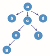
When introducing the conditions of tree structure, a special node root is mentioned. The root of the tree structure shown in the figure above is node A. just like a tree, a tree cannot grow dense branches and leaves without its roots. The formation of tree structure is also inseparable from the root node, but the tree grows upward, and the tree structure is depicted from the root down. It can be found in the figure above that there are no more nodes above the root node.
In addition to the root node a, the tree structure in the above figure also has nodes b, c, d, e, f and g. what they have in common is that there will be at least one node connected to it, both above and below the node. And in order to end the tree structure, we must ensure that there are no subsequent nodes, such as nodes b, d, f, G in the graph. Otherwise, it will become an infinite tree structure.
7.2 representation of tree
There are four forms of tree representation: tree representation, venturi diagram representation, concave representation and bracket representation. Next, we will introduce them one by one.
Tree representation
This is the most basic representation of the tree. An inverted tree similar to the one shown in the figure below is used to represent the tree structure, which is very intuitive and visual.

Venn's diagram representation
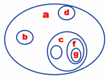
Venn's graph, also known as Venn's graph, Wynn's graph, Wien's graph and fan's graph, is suitable for representing the general relationship between sets (or) classes. It can also be used to represent the tree structure. For example, the tree structure shown above is shown in the figure below.
Concave representation
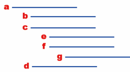
The concave representation uses the expansion and contraction of line segments to describe the tree structure, for example:
Bracket notation
The bracket representation is to write the root node of the tree structure on the left of the bracket, and the other nodes except the root node are written in the bracket and separated by commas. For example,

The diversity of representations shows the importance of tree structure in daily life and computer programming. Generally speaking, hierarchical classification schemes can be represented by hierarchical structure, that is, they can form a tree structure.
7.3 terms related to trees
Some terms are often used when explaining the operation of the tree later. This section briefly introduces some common terms first. Refer to the tree structure shown in the following figure:
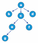
- Node: the blue ball shown in the figure above is called a node.
- Subtree: a tree formed by taking the child node of a node as the root, which is called the subtree of the node. Node a in the figure above, whose child node is c, and the tree with c as the root is called the subtree of node a. It is similar to the branches and leaves on the bifurcation of a tree in life.
- Branch: the relationship between nodes, similar to branches in life.
- Degree: the number of subtrees owned by a node is called the degree of the node. Node a in the figure above has three nodes b, c and d in its next layer (successor), so the degree of node a is 3.
- Parent node: the upper level (precursor) node of each node. The parent node of node e in the figure above is c and the parent node of node c is a.
- Root node: there is no upper level (precursor) node. A tree structure has only one root node. Node a in the figure above is the root node.
- Child node: the next (successor) node of a node. Nodes e and f in the figure above are the child nodes of node c.
- Leaf node: there is no next level (successor) node, which is called leaf node. The degree of leaf node is 0. Nodes b, g, f and d in the figure above are leaf nodes.
- Degree of tree: the maximum degree of all nodes in the tree, which is called the degree of tree. As shown in the figure above, the degree of a is 3, the degree of c is 2, the degree of e is 1, and the maximum degree is 3. Therefore, the degree of the whole tree structure is 3.
- Level (level number): the sum of the degrees of all nodes in the tree plus 1. The hierarchy shown in the above figure is: 3 × 1+2 × 1+1 × 1 + 1 = 7, so the level of this tree structure is 7.
- Sibling node: a node with the same parent node is called a sibling node. b, c and d in the figure above are sibling nodes.
- Depth: the maximum level of the node in the tree, which is called the depth of the tree. The tree structure in the figure above has four layers in total, and its depth is 4.
- Forest: the collection of complementary and intersecting trees is called forest. Similar to life, many big trees form a forest.
Binary tree is a special tree, which is more suitable for computer processing. Any tree can be converted into binary tree for processing. Next, we will focus on the binary tree structure.
7.4 what is a binary tree
Binary tree is still a tree structure, and it also applies to some related terms introduced in the previous section. However, a binary tree has another condition: each node has two branches, and the left branch is called the left subtree; The right branch is called the right subtree, so the maximum degree of a binary tree is 2. As shown in the figure:
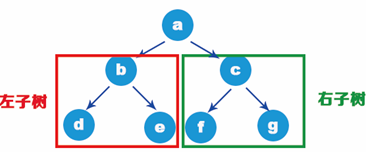
Binary tree has the following basic characteristics:
- In the k-th layer of binary tree, there are at most 2k-1 nodes. For the first layer in the figure above, k=1 is brought into the formula: 2k-1=21-1=1, then the first layer has at most one node; On the second floor in the figure, k=2 is brought into the formula: 2k-1=22-1=2. There are at most two nodes on the second floor. On the third floor in the figure, k=3 is brought into the formula: 2k-1=23-1=4. There are at most 4 nodes on the third floor.
- A binary tree with a depth of M has a maximum of 2m-1 nodes. For example, the depth of the binary tree in the figure above is 3, i.e. m=3, which is brought into the formula: 2m-1=23-1=7. The whole tree structure has up to 7 nodes.
- In any binary tree, the nodes with degree 0 are always 1 more than those with degree 2. As shown in the figure, there are 4 nodes with degree 0, d, e, f and g, and 3 nodes with degree 2, a, b and c. This tree structure has 1 more node with degree 0 than that with degree 2.
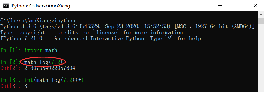
- The depth of a binary tree with n nodes is at least [log2n]+1. For example, there are seven nodes in the figure, and the formula is brought in: log2n= log27. After rounding, it is 2, and then 1 equals 3. Therefore, the tree structure has at least three layers.
7.5 binary tree category
There are several special types of binary trees: full binary tree, complete binary tree, skew binary tree and balanced binary tree. Next, let's introduce them one by one.
Full binary tree
Except for the leaf node of the last layer, the other nodes of the full binary tree have two nodes, that is, the nodes of each layer are full, as shown in the figure below:
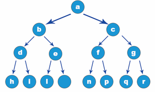
In the full binary tree, the k(k ≥ 0) layer has 2k-1 nodes, for example, when k=3, there are 23-1 = 4 nodes. A full binary tree with a depth of M has 2m-1 nodes. For example, when the depth is 4, there are 24-1 = 15 nodes. The depth of a full binary tree with n nodes is [log2n]+1. For example, when the node is 15, the depth is: [log215]+1=4.
Complete binary tree
The difference between a complete binary tree and a full binary tree is that except for the last layer, the nodes of each layer are full, and the last layer lacks only a few nodes on the right. As shown in the figure:
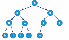
A full binary tree can be said to be a complete binary tree, while a complete binary tree cannot be said to be a full binary tree. The depth of a complete binary tree with n nodes is [log2n]+1.
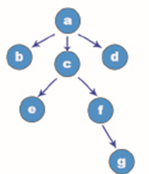
Skew binary tree
When a binary tree has no right or left nodes at all, it is called left skew binary tree or right skew binary tree. The first figure shows the left skew binary tree and the second figure shows the right skew binary tree.


As can be seen from the above two figures, the number of nodes in each layer of the skew binary tree is 1, there are n nodes, and the depth of the binary tree is n.
balanced binary tree
The balanced binary tree is neither a full binary tree nor a complete binary tree. The height difference between the left and right subtrees of the balanced binary tree is no more than 1. As shown in the figure below, it is a balanced binary tree.
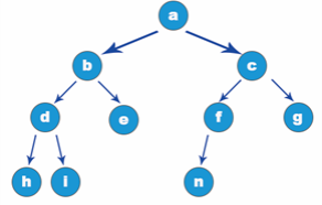
Note: empty binary tree is a binary tree without nodes. Empty binary tree is also a kind of balanced binary tree. Binary tree is a special tree, which is more suitable for computer processing. Any tree can be converted into binary tree for processing.
7.6 concept of reactor
Heap sort is a sort algorithm designed by using the data structure of heap. Heap is a structure similar to a complete binary tree, and satisfies the nature of heap at the same time: that is, the key value or index of a child node is always less than (or greater than) its parent node. From this sentence, the heap has two conditions:
- Is a complete binary tree.
- The key value or index of a child node is always less than (or greater than) its parent node.
Let's start with the first condition: complete binary tree. A complete binary tree (as mentioned above) is like a tree, except that each node of the binary tree has only two forks, and the generation order of the complete binary tree is from top to bottom and from left to right. As shown in the figure below, it is a complete binary tree.
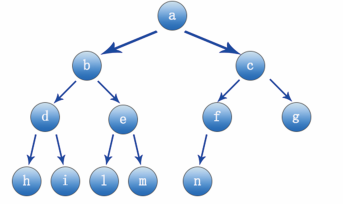
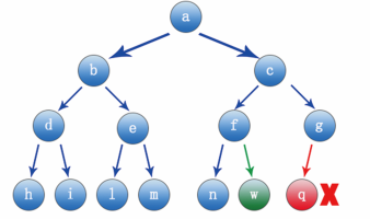
Where node a is the parent node of node b and c, node b is the parent node of d and e.. Conversely, nodes b and c are the child nodes of node a, and nodes d and E are the child nodes of node b For example, as shown in the following figure, if you want to add a node to the position of node q, it is wrong and does not meet the characteristics of a complete binary tree; The position of adding node w can meet the condition of complete binary tree.
Next, let's look at the second condition of the heap. The key value or index of the child node is always less than (or greater than) its parent node. For example, as shown in the following figure, there is a complete binary tree:
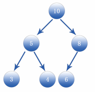
As can be seen from the above figure, parent node 10 is larger than its child nodes 5 and 8, while parent node 5 is larger than its child nodes 3 and 4, and parent node 8 is larger than its child node 6. It can also be seen from the figure that it is a complete binary tree, which also meets the requirement that the child node is larger than the parent node. Such a structure is called heap. According to the characteristics of the heap structure, the positions of the parent and child nodes of a node (for example, the node position is i) can be determined through a formula. The formula is as follows:
Formula for finding parent node:
Parent node location=(i-1)/2
 Formula for finding child nodes:
Left child node=2*i+1
 Right child node=2*i+2
For example, number the heap structure in the figure above, as shown in the figure below:
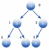
To require node 5 (its number is i=1), the formula brought in by the parent node is as follows:
Parent node location=(1-1)/2=0 # The data for position 0 is 10
Then find the position of the two sub nodes and bring in the formula as follows:
Left child node=2*1+1=3        # The data for position 3 is 3
 Right child node=2*1+2=4        # The data for position 4 is 4
7.7 sorting with heap
It can be seen from the above sorting algorithms that the fundamental process of sorting method is exchange. No matter which sorting method is selected, it is inseparable from the exchange of data. The same is true for heap sorting, which also needs to exchange data. Similarly, heap sorting also has two sorting results, namely, increasing sequence and decreasing sequence. The specific sorting processes of the two result forms are briefly described below:
- Ascending arrangement: the value of each node is greater than or equal to the value of its child nodes.
- Descending order: the value of each node is less than or equal to the value of its child nodes.
Next, a set of data is used to explain the heap sorting method in detail. For example, there is such a set of data 96, 54, 88, 5, 10 and 12, as shown in the figure:

Sort in ascending order as follows:
Step 1: put the data in the above figure into a complete binary tree structure, as shown in the following figure:
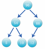
Step 2: exchange data according to the characteristics of the heap. The parent node is larger than the child node. From the above figure, the data of each parent node is larger than its own child node. Therefore, the parent node 96 is the maximum value of the data. At this time, it is necessary to exchange the rightmost data of the lowest layer of the complete binary tree with the parent node, that is, data 12 and 96, as shown in the figure:
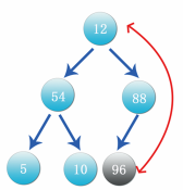
Step 3: after the exchange in the figure above, cut off the data 96 branches and put them into the sorted sequence, as shown in the figure below:
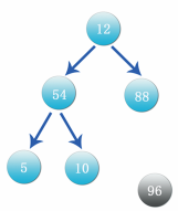
Step 4: again, observe that the parent node 12 is compared with its child nodes 54 and 88. First, compare the left node and find that 54 is greater than 12. Exchange the positions, as shown in the figure below. After the exchange, let's look at the branch with data 12 as the parent node. Its child nodes 5 and 10 are smaller than 12, so the location does not need to be exchanged.
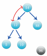
Step 5: compare the parent node 54 with its child nodes 12 and 88. 88 is larger than 54, and then exchange the positions of 54 and 88, as shown in the following figure:
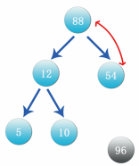
Step 6: after the exchange, 88 is the parent node, which is currently the largest number. Exchange the number 88 with the data 10 on the right at the bottom of the current complete binary tree. After the exchange, cut off the 88 branch and put it in front of 96. This process is shown in the following figure:
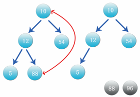
Step 7: at this time, data 10 is the parent node. Compare it with its child nodes 12 and 54 again. Compare the left child node. 12 is larger than 10. Exchange the positions of data 10 and 12, as shown in the figure below. After the exchange, look at the branch with 10 as the parent node. Its child node 5 is less than 10, so there is no need to exchange positions.
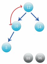
Step 8: when comparing with the right node, the data 54 is greater than 12, compare the data 12 with 54, as shown in the figure:
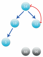
Step 9: after exchanging the status shown in the above figure, 54 is the current maximum value. Once again, it is necessary to exchange data 54 with data 5 at the bottom and right of the complete binary tree, cut off 54 branches and put them in front of data 88. The process is shown in the following figure:
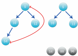
Step 10: as shown in the figure above, take 5 as the parent node, compare with its child nodes 10 and 15, and exchange the left child node first, as shown in the figure below:
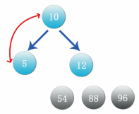
Step 11: compare the right node 12 again. If 12 is greater than 10, exchange the position, as shown in the following figure:
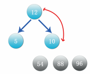
Step 12: at this time, the data 12 is the maximum value. Exchange the data with the lowest and rightmost data 10, cut off the branch of data 12 and put it in front of data 54, as shown in the figure:
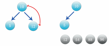
Step 13: at this time, only data 10 and 5 are left. The binary tree in the above figure also meets the heap, so put 10 directly in front of data 12 and 5 in front of data 10. The final result is shown in the following figure:

At this time, the heap sorting method has been used to sort the disordered data incrementally. In terms of steps, the parent node and child node are used to compare and exchange each time, and then Python is used to realize heap sorting.
[Example 7] use heap sorting method to sort the numbers in the list incrementally. The specific codes are as follows:
"""
Function name: heapify
 Function: adjust the elements in the list and ensure that i Is the heap of the parent node and ensures that i Is the maximum
 Parameter Description: heap: Represents the heap
          heap_len: Indicates the length of the heap
          i: Indicates the location of the parent node
"""


def heapify(heap, heap_len, i):
    """
    The subscript of a given node i,The subscripts of the parent node, left child node and right child node of this node can be calculated
    Parent node:(i-1)//2
    Left child node: 2*i + 1
    Right child node: 2*i + 2  That is, the left child node + 1
    """
    left = 2 * i + 1  # Left child node position
    right = 2 * i + 2  # Right child node position
    larger = i  # Each time the maximum value is assigned to the variable larger
    # The position of the left node is less than the length of the heap, and the maximum value of the heap is less than the value of the left child node
    if left < heap_len and heap[larger] < heap[left]:
        larger = left  # At this time, the node will be given the left position
    # The position of the right node is less than the length of the heap, and the maximum value of the heap is less than the value of the right child node
    if right < heap_len and heap[larger] < heap[right]:
        larger = right  # At this time, give the right node position to larger
    if larger != i:  # If heap adjustment is made, the value of larger is equal to the value of the left node or the right node
        heap[larger], heap[i] = heap[i], heap[larger]  # Do heap adjustment at this time
        # Recursively adjust each branch
        heapify(heap, heap_len, larger)


def build_heap(heap):  # Construct a heap and reorder all data in the heap
    heap_len = len(heap)  # heapSize is the length of the heap
    for i in range((heap_len - 2) // 2, - 1, - 1): # bottom-up reactor building
        heapify(heap, heap_len, i)


def heap_sort(heap):  # Take out the root node and swap with the last one, and continue the heap adjustment process for the first len-1 node
    build_heap(heap)  # Call function to create heap
    # The first element of the adjusted list is the largest element in the list. Exchange it with the last element, and then recursively adjust the remaining list to the maximum heap
    for i in range(len(heap) - 1, -1, -1):
        heap[0], heap[i] = heap[i], heap[0]
        heapify(heap, i, 0)


data = [96, 54, 88, 5, 10, 12]
print("The original data are:")
for k in range(6):  # Traverse the original data
    print('%4d' % data[k], end='')  # Output results
print('\n---------------------------')
print("The result after sorting is:")
heap_sort(data)
for k in range(6):  # Traversing sorted data
    print('%4d' % data[k], end='')  # Output results
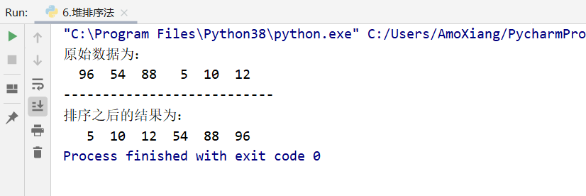
The operation results are shown in the figure below:
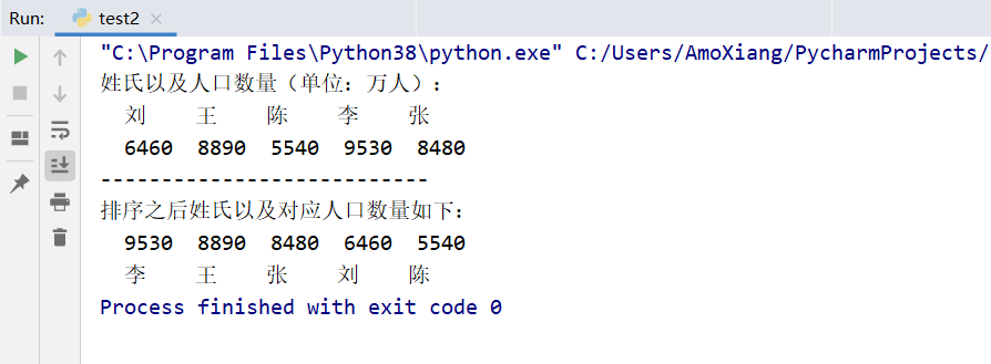
 [exercise 6] exercise: ranking of surnames. Hundreds of surnames have been memorized since childhood: Zhao, Qian, sun, Li, Zhou, Wu, Zheng, Wang... But I have seen a news before. According to the ranking of surnames with the largest population in China, it is not in this order. Next, the surnames are ranked according to the number of population. The specific codes are as follows:
"""
Function name: heapify
 Function: adjust the elements in the list and ensure that i Is the heap of the parent node and ensures that i Is the minimum value
 Parameter Description: heap: Represents the heap
          heap_len: Indicates the length of the heap
          i: Indicates the location of the parent node
"""


def heapify(heap, heap_len, i):
    """
        The subscript of a given node i,The subscripts of the parent node, left child node and right child node of this node can be calculated
        Parent node:(i-1)//2
        Left child node: 2*i + 1
        Right child node: 2*i + 2  That is, the left child node + 1
        """
    left = 2 * i + 1  # Left child node position
    right = 2 * i + 2  # Right child node position
    minimum = i  # Assign the minimum value to the variable minimum every time
    # The position of the left node is less than the length of the heap, and the minimum value of the heap is greater than the value of the left child node
    if left < heap_len and heap[minimum] > heap[left]:
        minimum = left  # At this time, the left node position is given to minimum
    # The position of the right node is less than the length of the heap, and the minimum value of the heap is greater than the value of the right child node
    if right < heap_len and heap[minimum] > heap[right]:
        minimum = right  # At this time, give the right node position to minimum
    if minimum != i:  # If heap adjustment is made, the value of minimum is equal to the value of the left node or the right node
        heap[minimum], heap[i] = heap[i], heap[minimum]  # Do heap adjustment at this time
        # Recursively adjust each branch
        heapify(heap, heap_len, minimum)


def build_heap(heap):  # Construct a heap and reorder all data in the heap
    heap_len = len(heap)  # heapSize is the length of the heap
    for i in range((heap_len - 2) // 2, - 1, - 1): # bottom-up reactor building
        heapify(heap, heap_len, i)


def heap_sort(heap):  # Take out the root node and swap with the last one, and continue the heap adjustment process for the first len-1 node
    build_heap(heap)  # Call function to create heap
    # The first element of the adjusted list is the largest element in the list. Exchange it with the last element, and then recursively adjust the remaining list to the minimum heap
    for i in range(len(heap) - 1, -1, -1):
        heap[0], heap[i] = heap[i], heap[0]
        heapify(heap, i, 0)


data = [6460, 8890, 5540, 9530, 8480]
data2 = ['Liu', 'king', 'Chen', 'Lee', 'Zhang']
print("Surname and population (unit: 10000):")
for datas2 in data2:
    print(" ", datas2, end='  ')
print()
for k in range(5):  # Traverse the original data
    print('%6d' % data[k], end='')  # Output results
print('\n---------------------------')
print("After sorting, the last name and the corresponding population are as follows:")
heap_sort(data)
for k in range(5):  # Traversing sorted data
    print('%6d' % data[k], end='')  # Output results
print()
data3 = ['Lee', 'king', 'Zhang', 'Liu', 'Chen']
for datas3 in data3:
    print(" ", datas3, end='  ')
The operation results are shown in the figure below:
8, Counting sorting method
The first seven sorting methods are based on the comparison and exchange of data, while the count sorting and cardinality sorting introduced next are non exchange sorting. In this blog post, let's take a look at the counting sorting method. The main idea of counting sorting is to convert the data values to be sorted into keys and store them in the extra array space. Counting and sorting requires that the input data must be integers with a certain range, so the counting and sorting method is applicable to data with a large amount and a small range, such as the entry years of employees, the age of employees, the ranking of college entrance examination, etc.
Next, a set of data is used to explain the counting sorting method in detail. For example, there is such a set of data 1, 2, 4, 1, 3, 5, 2, 2, 7, 3 and 4, as shown in the following figure:

Sort in ascending order as follows:
Step 1: check the maximum and minimum values of the original data to determine the range. The maximum value in the above figure is 7, so the range is from 0 to 7. Then prepare 8 barrels and number the barrels, as shown in the figure:

Step 2: put the corresponding numbers into each bucket in turn and start counting. For example, the first number 1 is put into bucket 1 and the counting number is 1; The second number is 2. Put it in bucket 2 and the count number is 1; The third number is 4, put it in bucket 4 and count the number 1; The fourth number is 1, which is still placed in barrel 1. At this time, the number of counts rises to 2, as shown in the following figure:

Step 3: according to the law of step 2, put the subsequent numbers into each bucket in turn and count the number. The final 7 buckets and the counted number are shown in the figure:

Take out the data from bucket No. 7, and then put it into bucket No. 1. For example, first remove the two numbers 1 in barrel 1, then take out the three numbers 2... In barrel 2, and take out all the data according to this law. The final result is shown in the figure:

From the results of the above figure, the data has been sorted, which is the process of counting sorting method. Next, the counting sorting method is implemented with Python code.
[example 8] use the counting sorting method to sort the numbers in the list incrementally. The specific codes are as follows:
def count_sort(data, maxValue):  # Define count sorting. Data is the list data and maxValue represents the maximum value
    bucket_len = maxValue + 1  # Defines that the length of the bucket is the maximum plus 1, and the bucket number starts from 0
    bucket = [0] * bucket_len  # Initialization bucket
    count = 0  # Count number
    arr_len = len(data)  # List length
    for i in range(arr_len):  # Traversal list
        if not bucket[data[i]]:  # List data is not bucket number
            bucket[data[i]] = 0  # At this time, initialize the bucket number of the list data from 0
        bucket[data[i]] += 1  # Add 1 to the bucket number in turn
    for j in range(bucket_len):  # Traversal bucket
        while bucket[j] > 0:  # Put the list data in the corresponding bucket number
            data[count] = j
            count += 1  # Count number plus 1
            bucket[j] -= 1  # The number is reduced by one, and the next same element is arranged forward
    return data  # Returns the sorted list


data = [1, 2, 4, 1, 3, 5, 2, 2, 7, 3, 4]
print("List data before sorting:")
for i in range(11):
    print("%2d" % data[i], end="")
print()
data2 = count_sort(data, 7)  # Call count sort function
print("Sorted list data:")
for j in range(11):
    print("%2d" % data2[j], end="")
The operation results are shown in the figure below:

From the above diagram as like as two peas, the final result is exactly the same as the result of the analysis just started.
9, Cardinal ranking method
The cardinal sort method, like the counting sort method, is a non commutative sort. Both cardinality sorting process and counting sorting process need to be carried out with the help of buckets. The main idea of cardinality sorting is to set several buckets, put the records with keyword K into the k-th bucket, and then connect the non empty data according to the sequence number. Keyword K is generated by dividing each data by one bit, ten bits, hundred bits. Cardinality sorting can be applied not only to the sorting between numbers, but also to string sorting (in 26 alphabetical order).
Next, a set of data is used to explain the cardinality sorting method in detail. For example, there is such a set of data 410, 265, 52, 530, 116, 789 and 110, as shown in the following figure:

Sort by increment, as follows:
Step 1: no matter the number of one digit, ten digit or hundred digit is composed of numbers 0 ~ 9, so the bucket number should also be from 0 ~ 9. For example, create a bucket, as shown in the figure:

Step 2: first classify the numbers in the original data by single digits, that is, the number 410 is 0, the number 256 is 6, and the number 52 is 2. According to this law, the single digits of this data are 0, 5, 2, 0, 6, 9 and 0 respectively, and put them in the corresponding bucket, as shown in the following figure:

Step 3: take out the data from each bucket according to the bucket number sequence. The sequence of fetched data is shown in the figure:

Step 4: classify the data taken from the above figure by ten digits, that is, the ten digits of 410 are 1530 and the ten digits of 1530 are 3. According to this law, the ten digits of this data are 1, 3, 1, 5, 6, 1 and 8 respectively, and put them in the corresponding bucket, as shown in the following figure:

Step 5: take out the data from each bucket according to the bucket number sequence. The sequence of fetched data is shown in the figure:

Step 6: classify the data taken from the above figure according to the hundred digits, that is, the hundred digit of 410 is 4110 and the hundred digit of 4110 is 1. According to this law, the hundred digits of this data are 4, 1, 1, 5, 0, 2 and 7 respectively, and put them in the corresponding bucket, as shown in the figure:

Step 7: take out the data from each bucket according to the bucket number sequence. The sequence of fetched data is shown in the figure:

From the results in the figure above, the data has been sorted, which is the process of cardinality sorting method. Next, the cardinality sorting method is implemented in Python code.
[Example 9] use the cardinality sorting method to sort the numbers in the list incrementally. The specific codes are as follows:
def radix_sort(data):  # Cardinality sorting. The parameter data is the sequence to be sorted
    i = 0  # The record is currently taking one position, and the lowest position is 1
    max_num = max(data)  # Maximum
    j = len(str(max_num))  # Number of digits to record the maximum value
    while i < j:
        # Initialize the bucket array. Since each digit is 0 ~ 9, create 10 buckets, and the list contains ten list elements
        bucket_list = [[] for x in range(10)]
        for x in data:  # Find data s
            bucket_list[int(x / (10 ** i)) % 10].append(x)  # Find the position and put it into the bucket array
        print(bucket_list)  # Print every barrel
        data.clear()  # Empty the original data
        for x in bucket_list:  # Put back the original data sequence
            for y in x:  # Traversing the sorted results
                data.append(y)  # Release data
        i += 1  # Execute once, and continue to take the data back to execute the loop


data = [410, 265, 52, 530, 116, 789, 110]  # List to be sorted
radix_sort(data)  # Call cardinality sort function
print(data)  # Output sorting results
The operation results are shown in the figure below:

From the results, there are ten lists in each row, representing barrels 0 ~ 9. The data contained in each list is the data put into the barrel in the above steps, which fully conforms to the steps explained above.
10, Comparison of various sorting algorithms in Python
10.1 entering the world of algorithms
10.1.1 what is an algorithm
Artificial intelligence is a popular word in today's era, which also makes many college students who want to make achievements in the field of artificial intelligence choose computer majors. Around us, there will be many examples of artificial intelligence applications. For example, in hospitals, doctors use AI to help diagnose whether patients have diseases; On the streets, the public sector uses robots to spray disinfectant; On the highway, traffic police use UAVs to patrol and dredge vehicles.
Artificial intelligence is a branch of computer. Naturally, it is inseparable from program language, which is very powerful (as shown in the figure below)

It can be used for Web development, game development, building scripts and GUI s for desktop applications, configuring servers, performing scientific calculations and data analysis. It can be said that the program language can be used to do almost anything! So why is the programming language so powerful? This is inseparable from the exquisite algorithm in the program. Therefore, behind a successful program, there must be a good algorithm.
At present, modern life has been very dependent on information technology. It seems that computers can do everything, but people who have a little understanding of the internal structure of computers will know that in fact, computers are just obedient. They don't know what they are doing. They will perform what actions users ask them to do. What can make the computer system omnipotent is a variety of algorithms, as shown in the figure:

The algorithm designed by human intelligence has created the intelligence of computer. Therefore, humans tell the computer in what order to perform certain actions, which is what we usually call algorithm.
If you want to go a long way in programming, you must have programming thinking. So what is programming thinking? Although computer related scholars do not have a clear definition so far, we can understand programming thinking as an adult way of thinking, and algorithm is a manifestation of computer programming thinking. From the current level of computer application, people have designed many very smart algorithms, which has greatly improved our ability to solve problems, but there are still many complex problems, and we still expect humans to give more effective algorithms.
10.1.2 function of algorithm
Algorithm is one of the core theories in computer science, and it is also one of the skills of human using computer to solve problems. Algorithms can be applied not only in the computer field, but also in some academic fields such as mathematics and physics. In fact, algorithms are used all the time in our life. For example, the chef's process of making delicious food, making work plans, designing exquisite page processes, etc. are all carrying out algorithm operations virtually. This section will introduce the function of the algorithm from the aspects of search information, communication, industry, mathematics and so on.
2.1 search information
Today is an era of big data coverage, and algorithms and data can evolve a variety of applications. For example, Baidu, our most familiar search engine, is shown in the figure below:
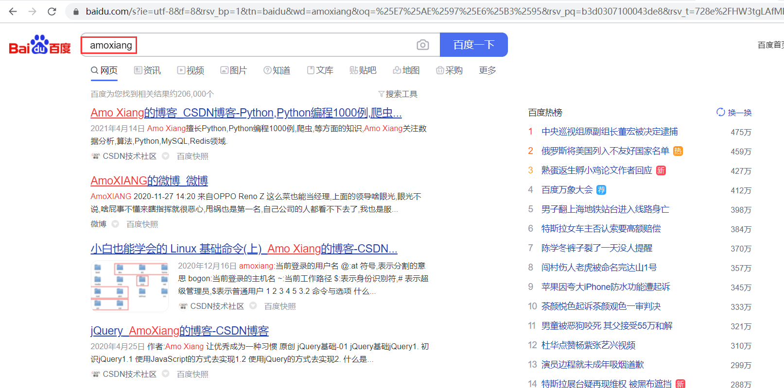
Efficient algorithms enable users to accurately find the information they want to search. Without these smart algorithms, users will be lost in the huge data forest of the Internet.
2.2 communication
The algorithm has made achievements not only in searching information, but also in communication. Without gifted coding and encryption algorithms, we can't communicate safely on the network, and the weather forecast can't be so accurate.
2.3 industry
Industrial production requires a lot of labor to promote the operation of the production line. How to manage the production line orderly, ensure product quality and improve production efficiency has become a hot topic; The top priority in industrial production. Through the use of a large number of precision algorithms, the industrial automation management system can intelligently manage, monitor, optimize and improve all links in production, as shown in the figure below:

2.4 mathematics
The great progress in the field of algorithms comes from beautiful ideas, which guide us to solve mathematical problems more effectively. Problems in the field of mathematics are not limited to arithmetic calculation. There are many problems that are not mathematicized on the surface, such as:
- How to sort
- How to find the shortest distance
- How to get out of the maze
- How to solve the Millennium Bug problem
These problems are very challenging. They need logical reasoning, geometry and combinatorial imagination to solve problems. These are the main abilities needed to design algorithms.
2.5 other aspects
In addition, many microprocessors contained in industrial robots, cars, aircraft and almost all household appliances rely on algorithms to function. For example, hundreds of microprocessors in the aircraft control the engine, reduce energy consumption and pollution with the help of algorithms; The microprocessor can control the brake and steering wheel of the car to improve stability and safety; Microprocessor can replace human beings to realize automobile driverless. The power of microprocessor is inseparable from perfect algorithm.
Therefore, the algorithm is very powerful. If you learn the algorithm well, you can write robust programs, and you won't be afraid of more severe challenges in your work.
10.1.3 basis of algorithm
Many people think that learning programming is to learn the latest programming language, technology and framework. In fact, computer algorithms are more important. From C language, C + +, Java to Python, although there are many kinds of programming languages, what remains unchanged is the algorithm. Therefore, only by cultivating the internal skill of algorithm and combining the moves of programming language can we dominate the programming Wulin. This section introduces the basis of the algorithm.
3.1 definition of algorithm
An algorithm is a set of instructions to complete a task, so some computer workers define it this way: in order to solve a certain or a certain kind of problem, it is necessary to express the instructions as a certain operation sequence. The operation sequence includes a group of operations, and each operation will complete a specific function. In short, the algorithm is a description of the steps to solve a specific problem, that is, the strategy to deal with the problem.
For example: the classic question - buy a hundred chickens for a hundred dollars. Note: from the analysis process to the implementation of the code in this blog post, the whole process is the process of the algorithm.
3.2 characteristics of the algorithm
Algorithm is to solve the problem of what to do and how to do. There may be different methods to solve a problem, but the core of algorithm analysis is the speed of the algorithm. Therefore, the steps to solve the problem need to be completed in a limited time, and there can be no ambiguous statements in the operation steps, so that the steps can not continue. Through the analysis of the concept of algorithm, it can be concluded that an algorithm must meet the following five characteristics. As shown in the figure below. This section introduces these five features.

-
Input. The algorithm and data in a program are interrelated. What needs to be input in the algorithm is the value of data. The input data can be multiple or zero. In fact, entering zero data does not mean that the algorithm has no input, but that the input is not intuitively displayed and hidden in the algorithm itself. For example, in Python language, the input() function is used to input data to the console. The code is as follows:
name = input("Please enter your name:") # Input variable value -
Certainty. The expression of each step in an algorithm should be determined. In people's daily life, when we encounter a sentence with unclear meaning, although it can be understood according to common sense and context, it may be misunderstood. As shown in the figure below, in Chinese social networking, acquaintances often ask, "have you eaten?" If you are a foreigner who does not understand Chinese culture, it is difficult to understand this sentence. What do you eat? having dinner? Eat fruit? I'm not sure who this question is about. This sentence has no certainty. It has neither subject nor object. People encounter such problems are difficult to understand, not to mention computers. The computer is no better than the human brain and will not guess the meaning of each step according to the meaning of the algorithm, so each step of the algorithm must have a definite meaning.

-
Output. The output is the result of the algorithm implementation. The algorithm is meaningless without output. Some algorithms output numerical values; Some output graphics, while others are not obvious. For example:
print("1314") # Output value print("^ _ ^") # Output graphics print(" ") # Output space, not obvious -
Limitation. An algorithm that can be implemented after a limited number of steps or can be completed in a limited time is called finite. For example, in the for loop of "buy a hundred chickens for a hundred dollars" (1,20), (1,33), (3,98,3), the limitation of this program is controlled. If there is no such condition, the for loop will loop endlessly, so the program will enter an endless loop, which does not meet the limitation of the algorithm.
Some algorithms are limited in theory and can be completed after limited steps, but in fact, the computer may execute for a day, a year, a decade or even longer. The core of the algorithm is speed, so this algorithm is meaningless. In short, there is no specific limit to finiteness, which mainly depends on the needs of users.
-
Effectiveness. The effectiveness of the algorithm means that each step can be executed effectively, and the determined results can be obtained. It can also be used to solve a class of problems conveniently. For example, z=x/y in the following program code is an invalid statement, because 0 cannot be used as the denominator.

3.3 algorithm performance analysis and measurement
Algorithm is the way to solve the problem. But there is more than one way to solve the problem. With more methods, there are naturally advantages and disadvantages. For example, when A person is sweeping the floor, people will not find that the person is good or bad. However, when two or three people do this work at the same time, people will have A comparison and can evaluate the quality of the work according to different evaluation criteria. Some people think A is good because he sweeps fast; Some people think B is good because he sweeps clean and waits.
So, how to evaluate the advantages and disadvantages of the algorithm? The following two aspects are introduced from the performance index of the algorithm and the measurement of algorithm efficiency.
Performance index of the algorithm
There are the following indexes to evaluate the advantages and disadvantages of an algorithm:
- Correctness: an algorithm must be correct before it has significance. This is the most important index. Programmers are required to use the correct computer language to realize the function of the algorithm.
- Friendliness: the function of the algorithm is for users. Naturally, it should have good usability, that is, user friendliness.
- Readability: the implementation of the algorithm may need to be modified many times or transplanted to other functions. Therefore, the algorithm should be readable and understandable to facilitate programmers to analyze, modify and transplant it to their own programs to realize some functions.
- Robustness: there are often unreasonable data or illegal operations in the algorithm, so an algorithm must be robust to check and correct these problems. When we first learn to write algorithms, we can ignore the existence of robustness, but we must make the algorithm more perfect through continuous learning.
- Efficiency: the efficiency of the algorithm mainly refers to the consumption of computer resources when executing the algorithm. Including the consumption of computer memory and computer running time. The two can be collectively referred to as space-time efficiency. It is meaningless for an algorithm to be only correct without efficiency. Generally, efficiency can also evaluate whether an algorithm is correct. If an algorithm needs to be executed for several years or even hundreds of years, the algorithm will be rated as wrong.
Measurement of algorithm efficiency
There are two ways to measure algorithm efficiency:
First, post calculation. First implement the algorithm, then run the program and calculate its time and space consumption. This measurement method has many disadvantages. Because the operation of the algorithm is related to the environmental factors such as computer software and hardware, it is not easy to find the advantages and disadvantages of the algorithm itself. The same algorithm compiles different object codes with different compilers, and the time required to complete the algorithm is also different. When the storage space of the computer is small, the running time of the algorithm will be prolonged.
Second, prior analysis and estimation. This measurement method evaluates the advantages and disadvantages of the algorithm by comparing the complexity of the algorithm. The complexity of the algorithm has nothing to do with computer software and hardware, but only with computing time and storage requirements. The measurement of algorithm complexity can be divided into space complexity measurement and time complexity measurement.
Time complexity of algorithm
The time complexity measurement of an algorithm is mainly to calculate the time used by an algorithm, mainly including program compilation time and running time. Since an algorithm can run many times once it is compiled successfully, the compilation time is ignored. Only the running time of the algorithm is discussed here.
The running time of the algorithm depends on the basic operations such as addition, subtraction, multiplication and division, as well as the data size, computer hardware and operating environment. Therefore, it is not feasible to calculate the time accurately. We can calculate the time complexity of the algorithm by calculating the main factor affecting the running time of the algorithm: the scale of the problem, that is, the amount of input.
Under the same conditions, the larger the scale of the problem, the longer the running time. For example, the algorithm for finding 1 + 2 + 3 +... + N, that is, the cumulative sum of N integers, the scale of this problem is n. Therefore, the time T required to run the algorithm is a function of the problem scale n, which is recorded as T(n).
In order to objectively reflect the execution time of an algorithm, the workload of the algorithm is usually measured by the execution times of the basic statements in the algorithm. This method of measuring time complexity is not a measure of time, but a measure of growth trend. When N changes, T(n) also changes. But sometimes we want to know what law it will take when it changes. Therefore, we introduce the concept of time complexity. In general, the number of times the basic operation is repeated in the algorithm is a function of the problem scale n, which is expressed by T(n). If there is an auxiliary function f(n), so that when n approaches infinity, the limit value of T(n)/f(n) is a constant that is not equal to zero, then f(n) is a function of the same order of magnitude of T(n). Note that T(n)=O(f(n)), and call O(f(n)) the progressive time complexity of the algorithm. This O(f(n)) representation is called large o (capital letter O) representation.
Spatial complexity of algorithm
The spatial complexity of the algorithm refers to the amount of auxiliary space required in the execution of the algorithm. The amount of auxiliary space does not refer to the storage space required by program instructions, constants, pointers, etc., nor the storage space occupied by input data. The auxiliary space is the storage space temporarily opened up by the algorithm in addition to the space occupied by the algorithm itself and the input and output data. The complexity of the algorithm in space (s) can be expressed as the complexity of the algorithm in time:
S(n) = 0(f(n))
For example, when the spatial complexity of an algorithm is a constant, that is, it does not change with the size of the processed data n, it can be expressed as O(1); When the spatial complexity of an algorithm is directly proportional to the logarithm of n based on 2, it can be expressed as O(log2n); When the spatial complexity of an algorithm is linearly proportional to N, it can be expressed as O(n).
10.1.4 large O representation
4.1 concepts and examples
Concept. Large o representation is a special representation, which represents the time complexity (i.e. speed) of the algorithm. Note: the big O representation is a rough estimate of the performance of an algorithm and cannot accurately reflect the performance of an algorithm.
give an example. Seeing this, you may have doubts about how the big O representation is expressed? Next, we use a program to introduce how the big O representation represents the time complexity of the program (please think about the following explanation from the perspective of function).
[example 1] calculate the values of a, b and c. For example: a+b+c=1000 and a2+b2=c2(a, b and c are natural numbers), find the possible combination of a, b and c (the range of a, b and c is between 0 and 1000). The code is as follows:
import time

start_time = time.time()
# Note that it is a triple cycle
for a in range(0, 1001):  # Traversal a
    for b in range(0, 1001):  # Traversal b
        for c in range(0, 1001):  # # Traversal c
            if a ** 2 + b ** 2 == c ** 2 and a + b + c == 1000:  # condition
                print("a, b, c: %d, %d, %d" % (a, b, c))
end_time = time.time()
print("elapsed: %f" % (end_time - start_time))
print("complete!")
Finally, it takes about 532 seconds (the running time of different computers is different) to run the results, as shown in the following figure:
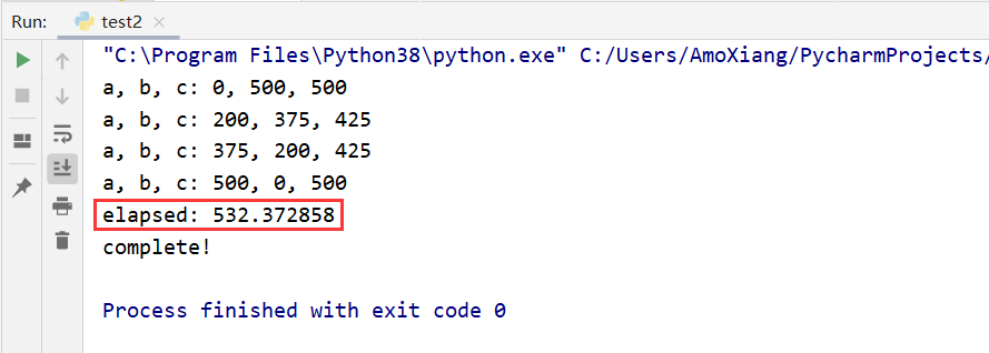
Modify the of this code as follows:
import time

start_time = time.time()
# Note that it is a triple cycle
for a in range(0, 1001):  # Traversal a
    for b in range(0, 1001):  # Traversal b
        c = 1000 - a - b  # Solving c with expression
        if a ** 2 + b ** 2 == c ** 2 and a + b + c == 1000:  # condition
            print("a, b, c: %d, %d, %d" % (a, b, c))
end_time = time.time()
print("elapsed: %f" % (end_time - start_time))
print("complete!")
The final running result of the second code takes less than 1 second, and the result is still the content shown in the figure above. In terms of speed, the second code is faster, that is, the algorithm of the second code is more mature and better than that of the first code. Let's analyze these two codes in terms of time:
-
Time complexity of the first code: set the time as f. this code uses three for loops. The time complexity of each loop traversing once is 1000, and the time complexity of three nested for loops is the time complexity of each layer of for loops multiplied, that is, T=1000*1000*1000. The if and print() statements after the for loop are counted as 2 for the time being. Therefore, the time complexity of this procedure is:
f = 1000 * 1000 * 1000 * 2
If the range of the for loop is written as 0~n, the time complexity becomes a function, where n is a variable, which can be written as follows, which is also equivalent to f(n)=n3*2:

The distribution of f(n)=n3*2 function in quadrant diagram is shown in the following figure:
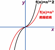
It can be seen from the image that the trend of this function is unchanged, and whether the coefficient is 2 or 1, it just makes the trend steeper and does not affect the general trend, so the coefficient 2 can be ignored. Then the trend shown in the image can basically be said to be the quadrant diagram of f(n)=n3, and the quadrant diagram formed by the increased coefficient is only the asymptote of f(n)=n3 (as shown in the red line above). The corresponding function is the asymptotic function. A series of asymptotic functions representing time complexity are represented by T(n), which becomes the following form (k represents coefficient):

As mentioned earlier, the coefficient k does not affect the trend of the function, so the value of k can be ignored here. Finally, T(n) can be written as follows:

This form is the large O representation, and f(n) is the large O representation of T(n). Where O(f(n)) is the time complexity of the asymptotic function of this code, referred to as time complexity, that is, T(n). Through the above analysis of the time complexity of the algorithm, it is concluded that when calculating the time complexity of any algorithm, all the coefficients of the lower power and the highest power can be ignored, which can simplify the algorithm analysis and focus on the growth rate. -
Time complexity of the second code: the second code has two layers of for loops, ignoring the coefficient. Its time complexity is T(n)=n2, and the final time complexity is f(n)=O(n2). The trend of the complexity of this code is shown in the figure below:
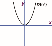
For example, such a code:
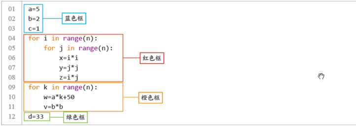
Find the time complexity T(n) of this code and analyze it as follows:
- The blue time complexity is T1(n)=3 (3 statements)
- The red time complexity is T2(n)=n*n*3=n2*3 (2-level for nested loop multiplied by 3 statements)
- The orange time complexity is T3(n)=n*2 (one layer for loop multiplied by two statements)
- The green time complexity is T4(n)=1 (1 statement)
- The time complexity of this program is T(n)= T1(n)+ T2(n)+ T3(n)+ T4(n)= 3+n2*3+n*2+1= n2*3+n*2+4
The form is derived from the large o representation (ignoring all coefficients of the lower and highest powers, including constants), and the final large o representation is T(n)=O(n2). The quadrant diagram is the same as that shown above. The common expressions of big O are as follows:
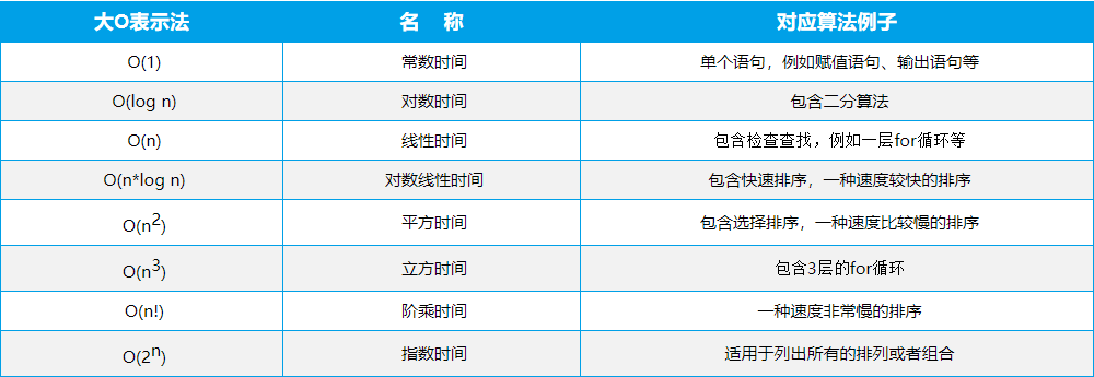
10.2 comparison of various sorting algorithms
In this blog post, nine sorting algorithms are introduced. What are the complexities of these nine sorting algorithms? This section summarizes the complexity and stability of various algorithms. Note: assuming that the length of the sequence to be sorted is n, the complexity of various sorting algorithms is shown in the following table:
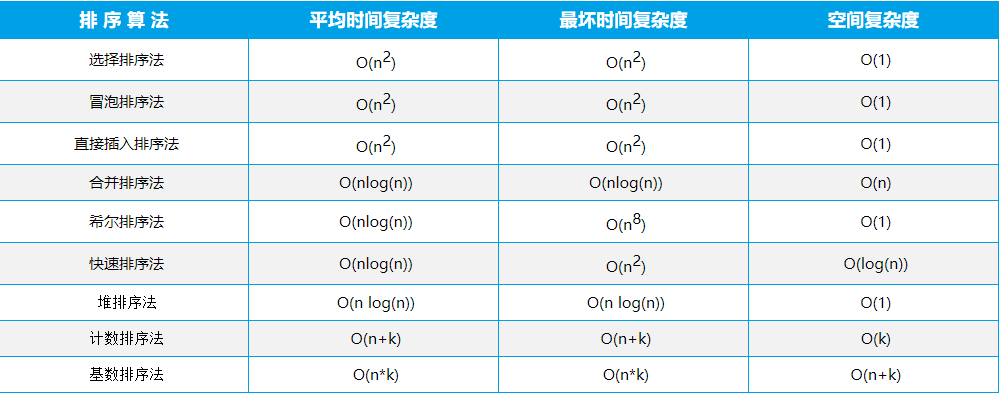
Learn two more tricks: auxiliary memory method: bubbling, selection and direct sorting require two for loops, focusing on only one element at a time, with an average time complexity of O (N2) (find element O(n) and position O(n) once). Fast, merge, hill is based on dichotomy, and the average time complexity is O (NLog (n)) (looking for element O(n) and location O(logn)). Counting sort and cardinal sort are linear order (O(n)) sort.