Multidimensional scaling (MDS) is a method to visualize the similarity level of multivariable samples (such as multiple species abundance and multiple gene expression). It carries out a series of ranking analysis based on distance matrix.
The classic MDS (CMDS) analysis is the PCoA analysis mentioned earlier, also known as metric MDS analysis. The opposite is non metric multidimensional scaling (NMDS).
Non metric multidimensional permutation (NMDS) is an indirect gradient analysis method based on dissimilarity matrix or distance matrix. The target of NMDS is similar to PCA or PCoA( Read PCA analysis (principle, algorithm, interpretation and visualization);Learn PCA/PCoA related statistical test (PERMANOVA) and visualization ), they all hope to show the relationship of samples in high-dimensional space as accurately as possible in low-dimensional space. In low dimensional space, the closer the distance between two sample points, the higher the similarity. The main purpose of NMDS is to identify and explain the distribution pattern of samples, reflect the sequential relationship between samples, and find gradient information that can show the source of sample differences, such as geographical environment information, ecological information, etc.
Different from MDS, NMDS analysis transforms the original distance matrix into rank matrix, and then carries out dimension reduction analysis. NMDS weakens the size of specific values in the distance matrix and pays more attention to their ranking relationship. If the distance between sample A and sample B is 5 and the distance between sample A and sample C is 10, the distance will not be described after conversion, but that sample B is the first closest to sample A and sample C is the second closest to sample A, and the ordered 1,2 is used to replace the original distance. Therefore, it is called "nonparametric" analysis.
NMDS can be applied to 1) data with missing pairing distance, 2) matrix generated by any distance algorithm, and 3) analysis of quantitative, semi quantitative, qualitative or mixed variables.
In the case of multiple samples and large number of species, NMDS model can more accurately reflect the numerical ranking information of distance matrix. Therefore, it is more accurate to use NMDS when there are too many samples or species.
NMDS is a continuous iterative process, through continuous attempts to find the most appropriate position of the sample in the dimensional space. The evaluation criterion is the stress value, which indicates the inconsistency between the observed distance and the fitted distance. Stress can also be understood as the difference between the distance of the space formed by the sample after dimensionality reduction and its distance in the original multidimensional space. The smaller the value, the better, indicating that the information of high-dimensional space is captured more completely in low-dimensional space. For NMDS two-dimensional analysis, it is generally considered that stress < 0.2 has certain explanatory significance; When stress < 0.1, it can be considered as a good ranking; When stress < 0.05, it has good representativeness.
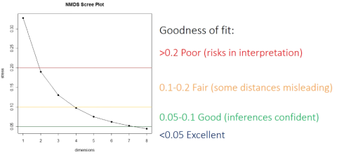
Before analysis, NMDS will select the number of dimensionality reduction axes and fit the data to the selected axes for sorting (the more axes, the less stress value; but the more axes, the more difficult it is to interpret). NMDS is different from other sorting algorithms in that its final solution is not unique, but attempts to obtain an acceptable solution many times. NMDS algorithm does not use factor decomposition techniques such as singular value singular vector, and NMDS1 and NMDS2 are not necessarily the axes that can explain the largest difference (but the difference explained by the first axis will be the largest in later analysis for better visualization). Therefore, the axis of NMDS can be converted on demand.
In biological information, NMDS is used to identify gene change patterns in time series expression profiles( https://www.biorxiv.org/content/10.1101/538918v1.full )And metagenomic data.
Metamds - recommended steps for NMDS analysis
NMDS is generally considered to be the most stable unrestricted ranking method in the field of Ecology (Minchin 1987). metaMDS is an NMDS analysis function in vagan that combines the analysis steps recommended by Minchin's (1987), which includes the following steps:
- Data conversion: when the parameter Autotransform = t (default), if the maximum abundance value in the input species abundance matrix (generally the flattened species abundance matrix) is greater than 9, Wisconsin double standardization will be carried out (the abundance value of each species will be divided by the maximum abundance of the species, and then the relative abundance will be calculated in each sample); If the maximum abundance value is greater than 50, the data will be square processed before Wisconsin conversion. If the data converted by yourself, such as the data converted by hellinger, does not want to be further converted, you can set autotransform = FALSE. If you enter a distance matrix, this step will also be skipped directly.
- Calculate dissimilarity matrix: the default is Bray Curtis, which is usually the best. Other distance matrices output by vegdist can also be selected. For non group data, we can use the function rankinex to find the most suitable matrix algorithm for our own data. If you enter a distance matrix, this step will also be skipped directly.
- Step across dissimilarities: if a large proportion of samples do not have common species, sorting will be difficult. In this case, it is necessary to calculate the shortest path between these different products instead of the difference value or distance between samples. The default NMDS engine function monoMDS can automatically deal with the situation of no shared species, and there is no need to call the stepacross function to calculate the shortest path. isoMDS, another engine function of NMDS, cannot automatically handle this situation. You need to set noshare=T to trigger the stepacross step. If you enter a distance matrix, this step will also be skipped directly.
- Multiple rounds of NMDS to find the optimal solution: NMDS will easily fall into the local optimum, and it is more likely to obtain the global optimal solution by running several times with different random start. The strategy of metaMDS is to run PCoA analysis first and use its results as a reference standard (RUN 0). If previous. Is set Best parameter, the NMDS result passed in by this parameter is used as a reference. Subsequently, metaMDS will set multiple random starting points to run NMDS analysis (the parameters try and trymax can set the minimum and maximum attempts). If the result of an NMDS is better than the current optimal result (the judgment standard is lower stress value), the result will be upgraded to the current optimal result and continue the cycle. You can set a value of trace = 2 or greater to track this optimization process. Set parallel=x to speed up the number of processes.
- Results Optimization: after obtaining the NMDS results, metaMDS was called postMDS to further optimize the results: 1) the results were integrated into the center of the coordinate axis. 2) Rotate NMDS1 according to the principal component to maximize the difference in the first dimension interpretation (you can also call the function MDSrotate to rotate the first axis parallel to the specified environment variable); 3) Community similarity units are equally divided.
- Species score: calculate the weighted score of species with the function wasscores in the final NMDS result.
Actual NMDS analysis
Continue to use the previous test data (for how to read your own data, see Above and When copying code, you always encounter the problem of what the original data should look like).
Note: the test data have been transposed. Each behavior is a sample and each column is a species; Their own data is usually one species / OTU per row and one sample per column, which needs to be transposed after reading.
library(vegan)
data("dune")
data("dune.env")

rownames(dune) <- paste0("Sample",1:nrow(dune))

# Transposition has been done. The samples are in the row and the species are in the column
head(dune)

##         Achimill Agrostol Airaprae Alopgeni Anthodor Bellpere Bromhord Chenalbu Cirsarve Comapalu Eleopalu Elymrepe Empenigr Hyporadi
## Sample1        1        0        0        0        0        0        0        0        0        0        0        4        0        0
## Sample2        3        0        0        2        0        3        4        0        0        0        0        4        0        0
## Sample3        0        4        0        7        0        2        0        0        0        0        0        4        0        0
## Sample4        0        8        0        2        0        2        3        0        2        0        0        4        0        0
## Sample5        2        0        0        0        4        2        2        0        0        0        0        4        0        0
## Sample6        2        0        0        0        3        0        0        0        0        0        0        0        0        0
##         Juncarti Juncbufo Lolipere Planlanc Poaprat Poatriv Ranuflam Rumeacet Sagiproc Salirepe Scorautu Trifprat Trifrepe Vicilath
## Sample1        0        0        7        0       4       2        0        0        0        0        0        0        0        0
## Sample2        0        0        5        0       4       7        0        0        0        0        5        0        5        0
## Sample3        0        0        6        0       5       6        0        0        0        0        2        0        2        0
## Sample4        0        0        5        0       4       5        0        0        5        0        2        0        1        0
## Sample5        0        0        2        5       2       6        0        5        0        0        3        2        2        0
## Sample6        0        0        6        5       3       4        0        6        0        0        3        5        5        0
##         Bracruta Callcusp
## Sample1        0        0
## Sample2        0        0
## Sample3        2        0
## Sample4        2        0
## Sample5        2        0
## Sample6        6        0

rownames(dune.env) <- paste0("Sample",1:nrow(dune.env))

# Perform NMDS recommended analysis steps through metaMDS
# k=2; Number of dimensions. NB., the number of points n should be n > 2*k + 1,
#     and preferably higher in global non-metric MDS, and still higher in local NMDS.
# try, tryamx: Minimum and maximum numbers of random starts in search of stable solution.
#     After try has been reached, the iteration will stop when two convergent solutions
#     were found or trymax was reached.
# autotransform: Use simple heuristics for possible data transformation of typical
#     community data (see below). If you do not have community data,
#     you should probably set **autotransform = FALSE**.
set.seed(1)
dune_nmds <- metaMDS(dune, distance="bray", k=2, try=20, trymax=50, autotransform=T,
                     model="global", stress=1, maxit=200, parallel=2, noshare=F)

## Run 0 stress 0.1192678
## Run 1 stress 0.1886532
## Run 2 stress 0.1192678
## ... Procrustes: rmse 5.822837e-06  max resid 1.845818e-05
## ... Similar to previous best
## Run 3 stress 0.1192678
## ... Procrustes: rmse 6.697234e-06  max resid 2.061976e-05
## ... Similar to previous best
## Run 4 stress 0.1183186
## ... New best solution
## ... Procrustes: rmse 0.02027078  max resid 0.06496407
## Run 5 stress 0.1192679
## Run 6 stress 0.1939202
## Run 7 stress 0.1808911
## Run 8 stress 0.1183186
## ... New best solution
## ... Procrustes: rmse 1.651369e-06  max resid 5.655239e-06
## ... Similar to previous best
## Run 9 stress 0.1192678
## Run 10 stress 0.1183186
## ... Procrustes: rmse 1.505928e-06  max resid 4.480433e-06
## ... Similar to previous best
## Run 11 stress 0.1192679
## Run 12 stress 0.1192678
## Run 13 stress 0.1886532
## Run 14 stress 0.1183186
## ... New best solution
## ... Procrustes: rmse 1.088269e-06  max resid 3.328672e-06
## ... Similar to previous best
## Run 15 stress 0.1192678
## Run 16 stress 0.1183186
## ... New best solution
## ... Procrustes: rmse 1.797827e-06  max resid 3.862713e-06
## ... Similar to previous best
## Run 17 stress 0.2075713
## Run 18 stress 0.1192678
## Run 19 stress 0.1192679
## Run 20 stress 0.1183186
## ... Procrustes: rmse 6.241246e-06  max resid 1.34356e-05
## ... Similar to previous best
## *** Solution reached
Obtained results: stress=0.118, the results are OK. (although autotransform=T is specified, this set of data does not trigger data conversion)
dune_nmds

##
## Call:
## metaMDS(comm = dune, distance = "bray", k = 2, try = 20, trymax = 50,      autotransform = T, noshare = F, model = "global", stress = 1,      maxit = 200, parallel = 2)
##
## global Multidimensional Scaling using monoMDS
##
## Data:     dune
## Distance: bray
##
## Dimensions: 2
## Stress:     0.1183186
## Stress type 1, weak ties
## Two convergent solutions found after 20 tries
## Scaling: centring, PC rotation, halfchange scaling
## Species: expanded scores based on 'dune'
If data conversion is done, there will be new data similar to the following:
Square root transformation Wisconsin double standardization ... global Multidimensional Scaling using monoMDS Data: wisconsin(sqrt(varespec))
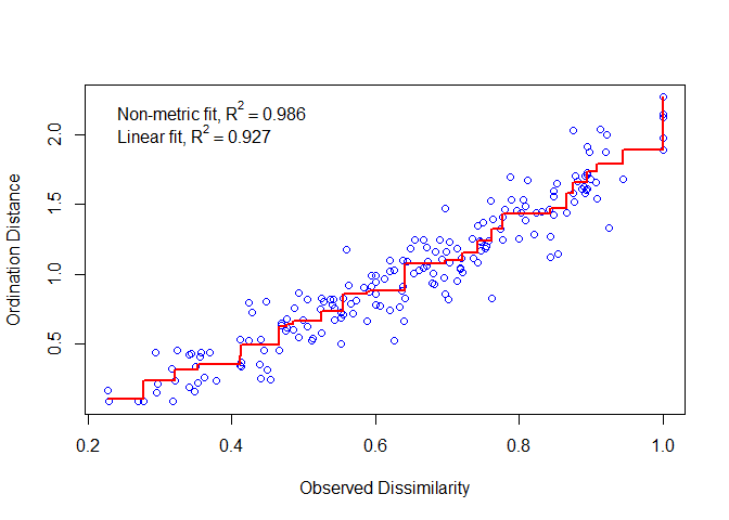
Ideally, the increased sorting distance is equal to the increased observation distance. All points fall on a monotonically increasing line. The more consistent, the better. If the deviation is large, the result is poor. The Stress value is the residual of the regression line in the figure below.
stressplot(dune_nmds)
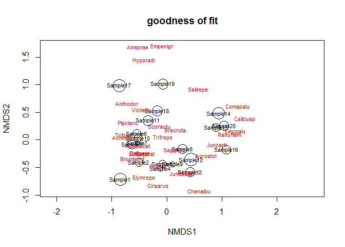
Calculate the fitting degree of each sample. The smaller the circle in the figure, the higher the fitting degree.
gof <- goodness(dune_nmds)
plot(dune_nmds, type="t", main = "goodness of fit")
points(dune_nmds, display="sites", cex=gof*100)
Sort out data and draw NMDS diagram.
dune_nmds_sample_result <- as.data.frame(scores(dune_nmds))
dune_nmds_sample_result$Sample <- rownames(dune_nmds_sample_result)
dune_nmds_sample_result <- cbind(dune_nmds_sample_result, dune.env)
dune_nmds_sample_result

##                NMDS1       NMDS2   Sample   A1 Moisture Management      Use Manure
## Sample1  -0.84054551 -0.71582776  Sample1  2.8        1         SF Haypastu      4
## Sample2  -0.50485425 -0.40893664  Sample2  3.5        1         BF Haypastu      2
## Sample3  -0.08267021 -0.43667531  Sample3  4.3        2         SF Haypastu      4
## Sample4  -0.11562467 -0.52223859  Sample4  4.2        2         SF Haypastu      4
## Sample5  -0.62654363 -0.08669513  Sample5  6.3        1         HF Hayfield      2
## Sample6  -0.54269773  0.11315559  Sample6  4.3        1         HF Haypastu      2
## Sample7  -0.54030010 -0.05820584  Sample7  2.8        1         HF  Pasture      3
## Sample8   0.28115518 -0.16683738  Sample8  4.2        5         HF  Pasture      3
## Sample9   0.11057585 -0.44257696  Sample9  3.7        4         HF Hayfield      1
## Sample10 -0.51697230  0.02738090 Sample10  3.3        2         BF Hayfield      1
## Sample11 -0.33831007  0.35081631 Sample11  3.5        1         BF  Pasture      1
## Sample12  0.44246800 -0.36410934 Sample12  5.8        4         SF Haypastu      2
## Sample13  0.41863051 -0.58334738 Sample13  6.0        5         SF Haypastu      3
## Sample14  0.94331987  0.47606816 Sample14  9.3        5         NM  Pasture      0
## Sample15  0.89599692  0.22235599 Sample15 11.5        5         NM Haypastu      0
## Sample16  1.08109124 -0.17966386 Sample16  5.7        5         SF  Pasture      3
## Sample17 -0.85990338  0.98711836 Sample17  4.0        2         NM Hayfield      0
## Sample18 -0.17720324  0.52341328 Sample18  4.6        1         NM Hayfield      0
## Sample19 -0.07001774  1.01213863 Sample19  3.7        5         NM Hayfield      0
## Sample20  1.04240524  0.25266697 Sample20  3.5        5         NM Hayfield      0

# Using the scores function from vegan to extract the species scores
# and convert to a data.frame
dune_nmds_species_result <- as.data.frame(scores(dune_nmds, "species"))
dune_nmds_species_result$Species <- rownames(dune_nmds_species_result)
dune_nmds_species_result

##                NMDS1       NMDS2  Species
## Achimill -0.82280076  0.04328704 Achimill
## Agrostol  0.71096003 -0.28924414 Agrostol
## Airaprae -0.52817837  1.67987383 Airaprae
## Alopgeni  0.39096747 -0.58596256 Alopgeni
## Anthodor -0.72021737  0.65914560 Anthodor
## Bellpere -0.47838087 -0.24446722 Bellpere
## Bromhord -0.61896693 -0.33475908 Bromhord
## Chenalbu  0.59187098 -0.92197922 Chenalbu
## Cirsarve -0.15184056 -0.82169646 Cirsarve
## Comapalu  1.28932838  0.60840015 Comapalu
## Eleopalu  1.24504861  0.16149275 Eleopalu
## Elymrepe -0.42014574 -0.68023468 Elymrepe
## Empenigr -0.08835329  1.69629767 Empenigr
## Hyporadi -0.41569548  1.44600334 Hyporadi
## Juncarti  0.91146010 -0.08309672 Juncarti
## Juncbufo  0.26476745 -0.60761447 Juncbufo
## Lolipere -0.51199146 -0.24807077 Lolipere
## Planlanc -0.70645212  0.32063694 Planlanc
## Poaprat  -0.38844035 -0.25091394  Poaprat
## Poatriv  -0.15906762 -0.47836751  Poatriv
## Ranuflam  1.14363918  0.09953894 Ranuflam
## Rumeacet -0.52479268 -0.10530738 Rumeacet
## Sagiproc  0.14315579 -0.18745689 Sagiproc
## Salirepe  0.57484082  0.91104875 Salirepe
## Scorautu -0.13956707  0.25000522 Scorautu
## Trifprat -0.77154453  0.08564591 Trifprat
## Trifrepe -0.07526697  0.04516674 Trifrepe
## Vicilath -0.46793995  0.54914931 Vicilath
## Bracruta  0.15071778  0.18979787 Bracruta
## Callcusp  1.42118155  0.38376646 Callcusp
NMDS is a scatter diagram. Each point in the graph usually represents the sample, and different colors / shapes represent the grouping information to which the sample belongs or other concerned sample attribute information. The distance between sample points in the same group indicates the repeatability of the sample, and the distance between samples between groups reflects the difference in the detection variable space. It is usually necessary to mark the stress information, not the weight information of the axis.
library(ggplot2)
library(ggalt)

p1 <- ggplot(data=dune_nmds_sample_result,
             aes(x=NMDS1,y=NMDS2,fill=Management,
                 colour=Management,group=Management)) +
  geom_point(size=3) + # add the point markers
  geom_encircle(alpha=0.1, show.legend = F) +
  geom_hline(aes(yintercept=0),color="grey", linetype=3) +
  geom_vline(aes(xintercept=0),color="grey", linetype=3) +
  labs(title=paste0("Stress: ", round(dune_nmds$stress,3))) +
  theme_classic()

p1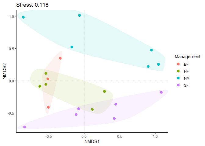
Map species information in NMDS two-dimensional space at the same time (it is messy when there are many species. You can screen some peak species and then screen dune_nmds_species_result for mapping. Or you can directly map species information.
p1 <- ggplot() +
  geom_point(data=dune_nmds_sample_result,
             aes(x=NMDS1,y=NMDS2,
                 colour=Management,group=Management),size=3) + # add the point markers
  geom_encircle(data=dune_nmds_sample_result,
                aes(x=NMDS1,y=NMDS2,fill=Management,group=Management),
                alpha=0.1, show.legend = F) +
  geom_hline(aes(yintercept=0),color="grey", linetype=3) +
  geom_vline(aes(xintercept=0),color="grey", linetype=3) +
  geom_point(data=dune_nmds_species_result, aes(x=NMDS1,y=NMDS2)) +
  geom_text(data=dune_nmds_species_result, aes(x=NMDS1,y=NMDS2,label=Species)) +
  labs(title=paste0("Stress: ", round(dune_nmds$stress,3))) +
  theme_classic()
p1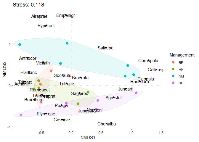
reference resources
- NMDS https://archetypalecology.wordpress.com/2018/02/18/non-metric-multidimensional-scaling-nmds-what-how/
- NMDS https://blog.csdn.net/weixin_53819139/article/details/114133818
- https://www.cd-genomics.com/microbioseq/non-metric-multidimensional-scaling-nmds-in-microbial-sequencing-data-analysis-introduction-application-and-comparison.html
- Good explanation of sorting concept http://albertsenlab.org/ampvis2-ordination/
- https://blog.csdn.net/woodcorpse/article/details/107032032?utm_medium=distribute.pc_aggpage_search_result.none-task-blog-2~aggregatepage~first_rank_ecpm_v1~rank_aggregation-4-107032032.pc_agg_rank_aggregation&utm_term=beta%E5%A4%9A%E6%A0%B7%E6%80%A7&spm=1000.2123.3001.4430
- https://mb3is.megx.net/gustame/dissimilarity-based-methods/nmds
- https://jkzorz.github.io/2019/06/06/NMDS.html
- https://mp.weixin.qq.com/s/3NtVtqhEinqtbh2B-qnktg
- https://mp.weixin.qq.com/s/uWX9CUBNR2ybJ1LxFhKefQ