preface

I Getting started with Numpy

NumPy (Numerical Python) is an open source numerical calculation extension of Python. It provides multidimensional array objects and various derived objects (such as mask arrays and matrices). This tool can be used to store and process large matrices, which is much more efficient than Python's own nested list structure (this structure can also be used to represent matrices), and supports a large number of dimensional arrays and matrix operations, In addition, it also provides a large number of mathematical function libraries for array operation, including mathematics, logic, shape operation, sorting, selection, input and output, discrete Fourier transform, basic linear algebra, basic statistical operation, random simulation and so on.

Almost all data analysts working in Python take advantage of the power of NumPy.
a. Powerful N-dimensional array
b. Mature broadcast function
c. Toolkit for integrating C/C + + and Fortran code
d.NumPy provides comprehensive mathematical functions, random number generator and linear algebra functions

1. Development environment installation and configuration

🚩 There are two different installation methods. This paper mainly introduces the second method and provides two download channels:

The first way:
Enter the following two lines in cmd:

pip install jupyter -i https://pypi.tuna.tsinghua.edu.cn/simple
pip install numpy -i https://pypi.tuna.tsinghua.edu.cn/simple

The second way:
Install Anaconda directly download: Anaconda Installers

Readers download according to their different operating systems. The blogger is Windows system. The following installation process is also carried out on Windows operating system, but there is little difference.

You can also download it directly from Baidu online disk: Anaconda Installers , extraction code: 3h2u




❗ Note: Add Path!!! Add environment variables~

Enter wait:

Installation complete~



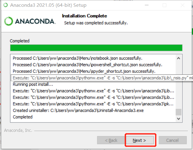
Two websites will pop up:

Don't worry, just close it.

We enter cmd and enter:

jupyter notebook

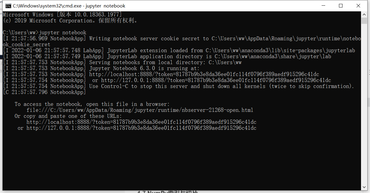
Then you will enter a website:

So far, our Anaconda installation is successful, and the integration~ 🎈

Let's create a new folder here:


At this time, the file is unnamed. Let's give it a name:



We create a python 3 in AIoT:

We still change its name:

So far, we have successfully created the python 3 file, conversion~ 🎈

2.NumPy array export

🚩 Let's start writing code:

After writing a line, we can click Run, and also use the shortcut key: Shift + Enter to run:

You can view all shortcut keys as follows:


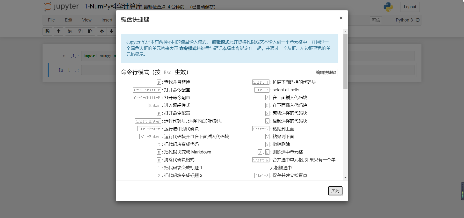
Our code can be run repeatedly: for example, if we run the first line of code again, we will find that it has changed from In [1] to In[2]:




Now let's turn it blue:


Ugly, right, because in Python syntax, # represents comments, and in Markdown, # represents first-class titles.
So we can remove it#


Press shortcut key: B to continue writing code

Doesn't it look awkward without a line number? Click View - > line numbers:

We write a code and output a list. We click Run:

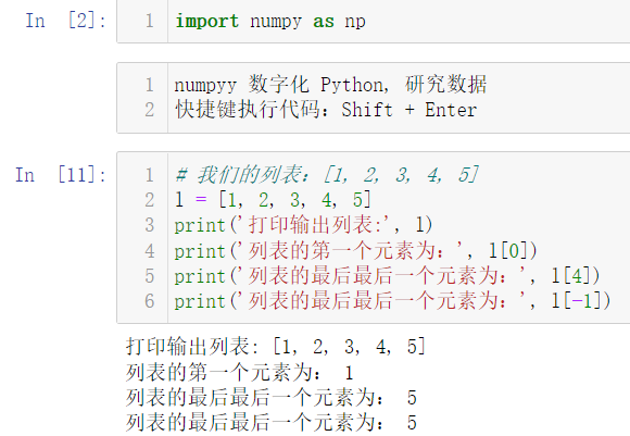
Of course, our slicing operation is the same:

Our protagonist is on the stage! numpy array


numpy arrays support simpler operations:
For example, in our list, the following operations will report errors:

However, our numpy array supports the above operations:

Of course, there are some "outrageous" operations:


Obviously, there is no such "operation" in our list:

3.NumPy array creation

🚩 In fact, we have briefly introduced how to create an array in 1.2 NumPy array export: using the array function
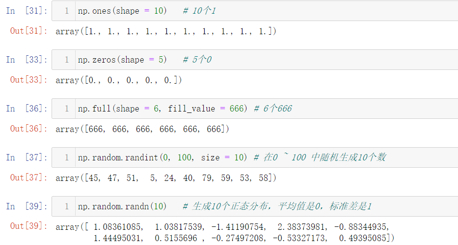
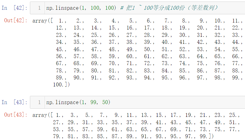
However, there are many ways to create (initialize) an array in NumPy:

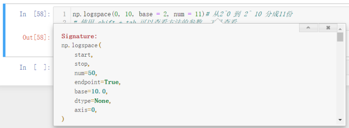
We find that we can't understand the running results of this logspace because it is expressed in scientific counting method. We can use NP set_ Printoptions (suppress = true) to make the running results into numbers that we can understand:



Above code:

np.ones(shape = 10)   # 10 1

np.zeros(shape = 5)   # 5 zeros

np.full(shape = 6, fill_value = 666) # 6 666

np.random.randint(0, 100, size = 10) # Randomly generate 10 numbers in 0 ~ 100

np.random.randn(10)   # Generate 10 normal distributions, with an average of 0 and a standard deviation of 1

np.linspace(1, 100, 100) # Divide 1 ~ 100 into 100 parts (arithmetic sequence)

np.linspace(1, 99, 50)

np.set_printoptions(suppress = True)
np.logspace(0, 10, base = 2, num = 11)# From 2 ^ 0 to 2 ^ 10 divided into 11 parts
# Use the shift + tab to view method parameters and tools

# Two dimensional array: 3 rows and 5 columns
np.random.randint(0, 10, size = (3, 5))

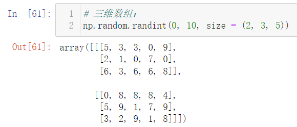
# 3D array:
np.random.randint(0, 10, size = (2, 3, 5))

4.NumPy array view

🚩 jupyter extension (or not installed)
Enter the following command in our cmd:

pip install jupyter_contrib_nbextensions -i https://pypi.tuna.tsinghua.edu.cn/simple
pip install jupyter_nbextensions_configurator -i https://pypi.tuna.tsinghua.edu.cn/simple
jupyter contrib nbextension install --user
jupyter nbextensions_configurator enable --user

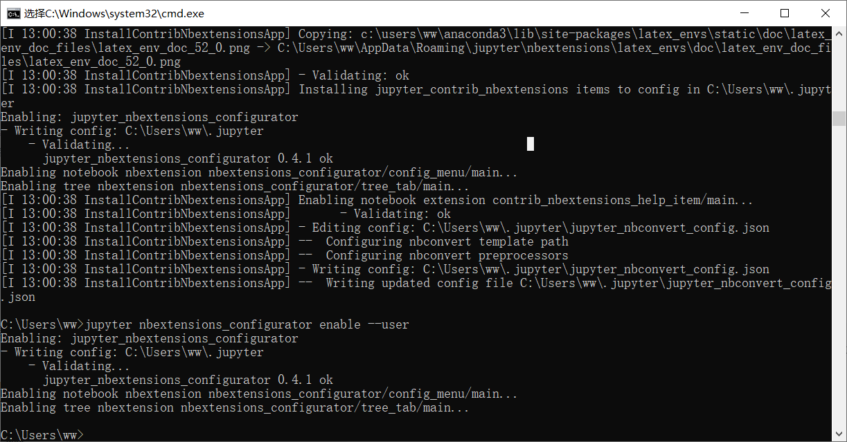
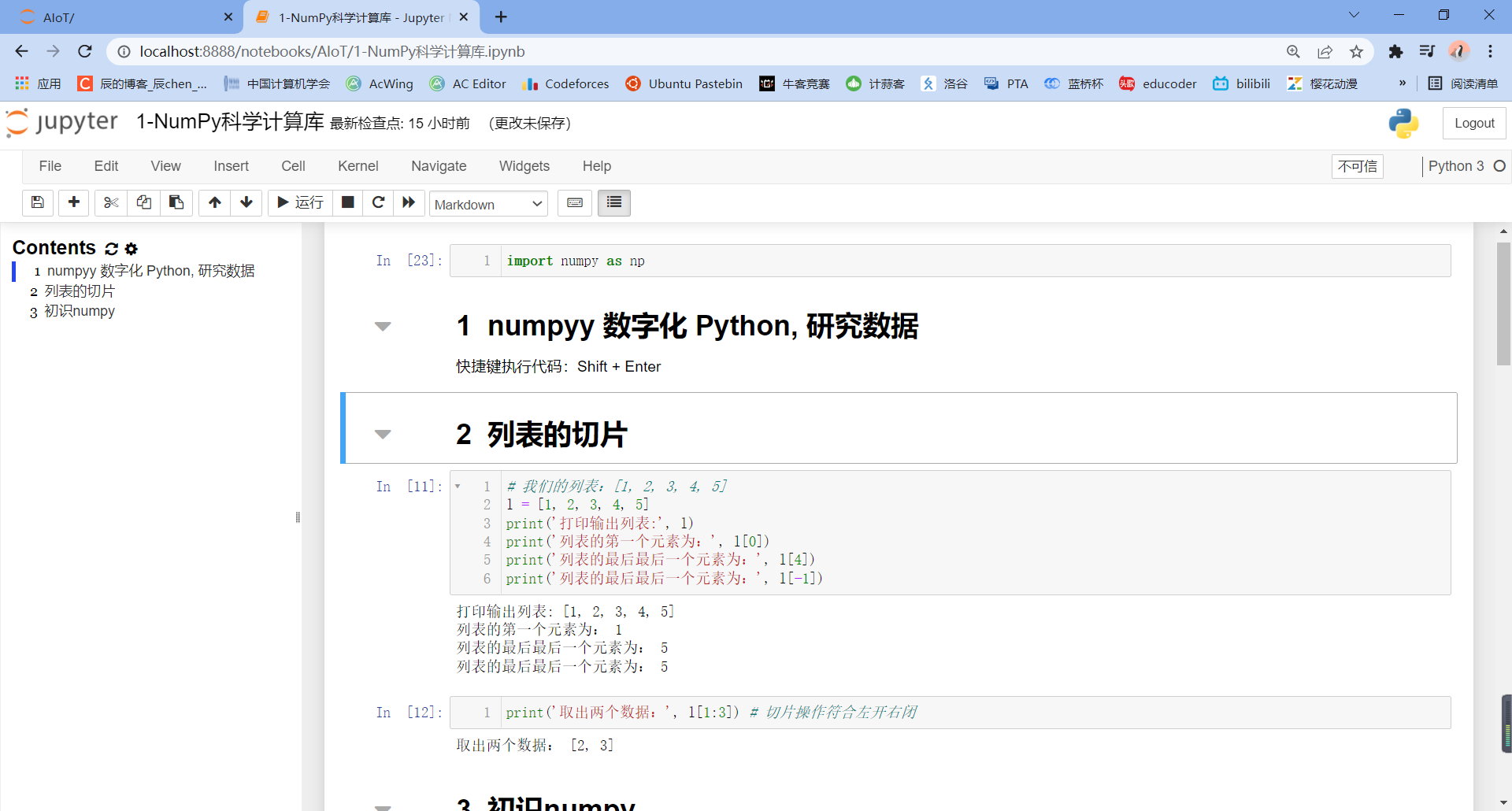
After installation, exit and re-enter the Jupiter Notebook:


Check the following:

After installation, enter our code again and you will find one more thing:

Click to display an index directory:

4.1 dimension of array

import numpy as np
arr = np.random.random(size = (3, 5))
arr.ndim    # dimension

4.2 shape of array

import numpy as np
arr = np.random.random(size = (3, 5))
arr.shape    # shape

4.3 total number of array elements

import numpy as np
arr = np.random.random(size = (3, 5))
arr.size    # Total number of array elements

4.4 data type

import numpy as np
arr = np.random.random(size = (3, 5))
arr.dtype   # Data type float64 (64 bit)

4.5 size of each element in the array (in bytes)

import numpy as np
arr = np.random.random(size = (3, 5))
# 0, 1 ----- > bit
# 8 bits ----- > bytes
# 64 / 8 = 8
arr.itemsize  # The size of each element, corresponding to 8 bytes

5.NumPy data saving

🚩 We can use the save method to save our array:

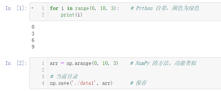
import numpy as np
arr = np.arange(0, 10, 3)    # NumPy's method has similar functions

# current directory
np.save('./data1', arr)      # preservation

After running, we return to the created Directory:

You can find one more data1 NPY here is the array information we just saved.

Note that if you click the newly created file, you will find:

There is no storage information we want to see. This is because the contents saved in the file are binary and can only be opened with code. Next, we introduce the method of reading our data from the file:

We can extract the data according to the following code:

import numpy as np
arr = np.arange(0, 10, 3)    # NumPy's method has similar functions
np.load('./data1.npy')       # Fetch data

If we want to save multiple arrays into one file, we can use the savez method:

import numpy as np
arr = np.arange(0, 10, 3)    # NumPy's method has similar functions
np.set_printoptions(suppress = True)
arr2 = np.logspace(0, 10, base = 2, num = 11)
np.savez('./data2.npz', x = arr, y = arr2) 
# Store both arr and arr2 in '/ data2.npz'
# Store the ARR in and call it x; Save arr2 and call it y

After running, you can see an additional data2 Npz file, which is the array information we just saved.

We can take values one by one:

import numpy as np
arr = np.arange(0, 10, 3)    # NumPy's method has similar functions
np.set_printoptions(suppress = True)
arr2 = np.logspace(0, 10, base = 2, num = 11)
np.load('./data2.npz')['x']   # Take out X -- > take out arr
np.load('./data2.npz')['y']   # Take out Y -- > take out arr2

Pay attention to what name we use when saving and what name we use when retrieving, for example:

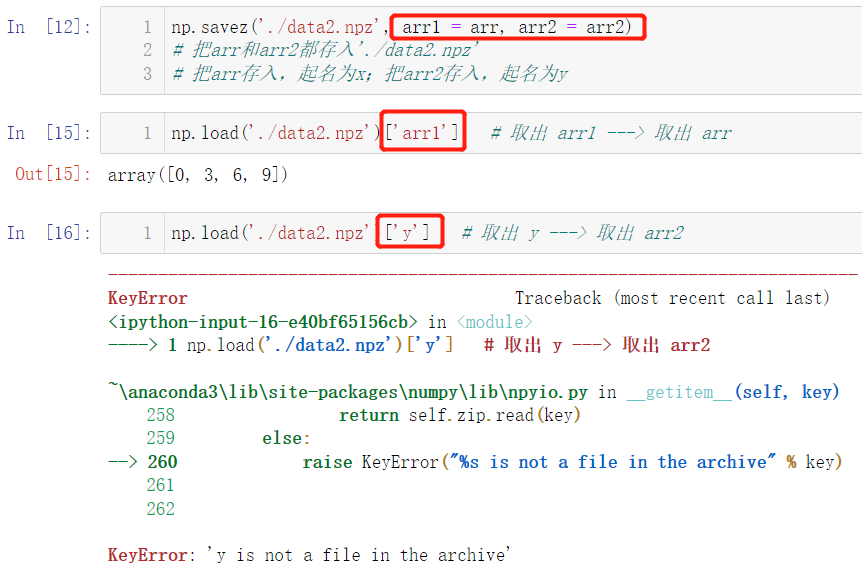
Obviously, taking y out at this time is wrong.

Read and write csv and txt files:

import numpy as np
arr = np.random.randint(0, 10, size = (3, 4))
# Save array to csv file 
np.savetxt("./arr.csv", arr, delimiter = ',')  # The same is true for storing to txt files
# read file
np.loadtxt('./arr.csv', delimiter = ',', dtype = np.int32)

6.NumPy data type

🚩 Our data types fall into three categories:

integer

Floating point number

character string

Data type of ndarray:

• Int (integer): int8, uint8, int16, int32, int64

• Float: float16, float32, float64

• str (string)

What is the difference between float16, float32, int16 and int 32: the larger the number, the larger the memory it occupies in the memory. Of course, the larger the range of numbers that can be represented: for example, the range of int8 is 28, but because it contains both positive and negative numbers, the range it can express is [- 128, 127], and the range of unit8 is 28, The difference is that it does not contain negative numbers, that is, it only contains 0 and positive numbers, so the value range of unit8 is [0, 255]. The data type can be converted by using the astype() method:
When we create a type, we can use dtype to indicate its data type

Of course, we can also give it int32:

We input the following code to compile and run:

Then go back to our folder and see the two files we just saved:

It is very intuitive to note that the size difference between the two files is approximately 8 times. The reason for this is actually 64 / 8 = 8

Use the astype() method to convert data types:

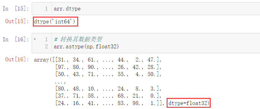
Here, we need to note that after conversion, the data type of the original array remains unchanged. Using astype() to convert can be said to create a new array:

7.NumPy array operation

🚩 Array operations include operations within an array element and operations between two or more arrays:

7.1 addition, subtraction, multiplication and division power operation

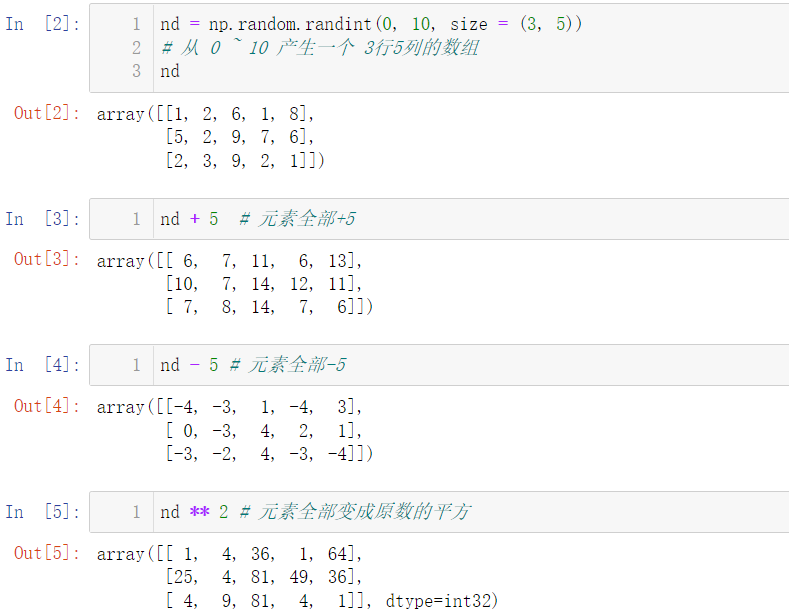
We can also call the power() function when calculating the power

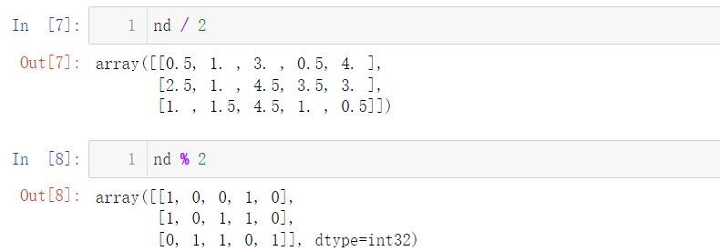
Of course, it also supports / and% operations

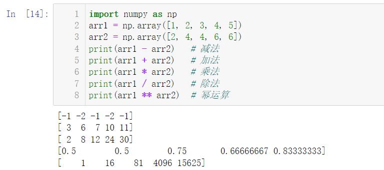
The operation of two arrays is actually the operation of corresponding positions:

import numpy as np
arr1 = np.array([1, 2, 3, 4, 5])
arr2 = np.array([2, 4, 4, 6, 6])
print(arr1 - arr2)   # subtraction
print(arr1 + arr2)   # addition
print(arr1 * arr2)   # multiplication
print(arr1 / arr2)   # division
print(arr1 ** arr2)  # exponentiation 

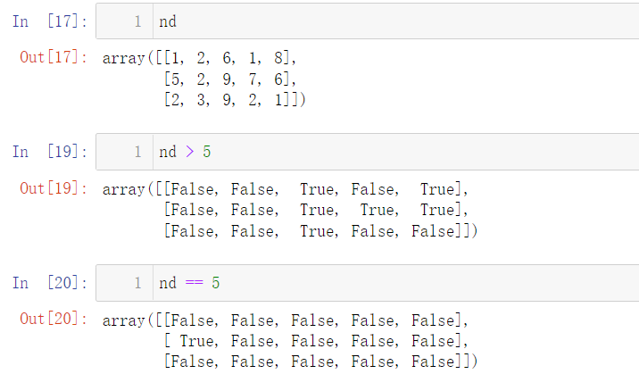
7.2 logic operation

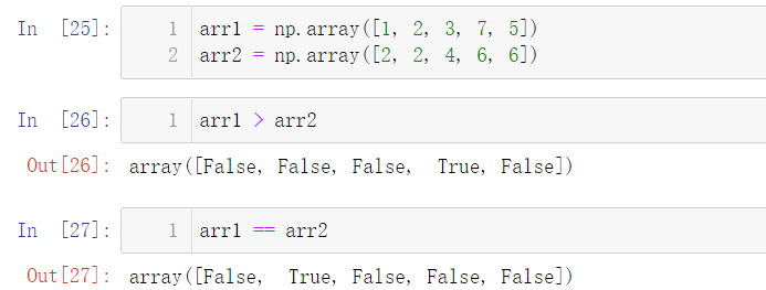
Of course, there are logical operations between the two arrays:

7.3 + = - = * = operation

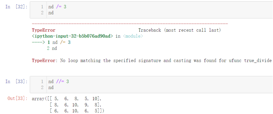
❗ Note: the above operations do not change the original value of the array, which can be understood as re creating a new array, but the following operations are directly modified on the basis of the array, which will change the value of the elements of the array

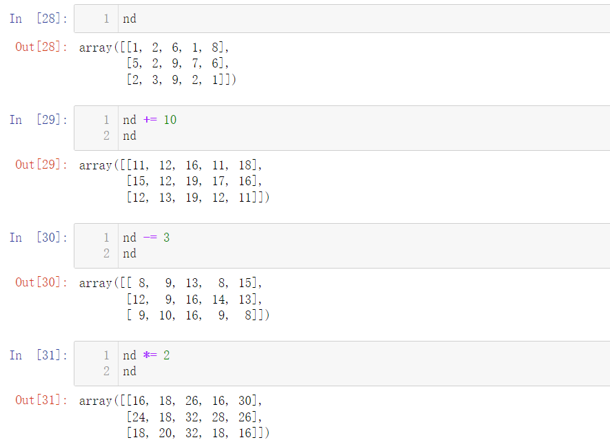
Note that / = operation is not included here, and an error will be reported. Here, it is / / =:

8.NumPy index and slice

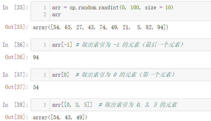
🚩 In fact, we often use index and slice operations in the list. We won't go into too much detail here. We will explain the implementation of index lookup and slice operations in NumPy

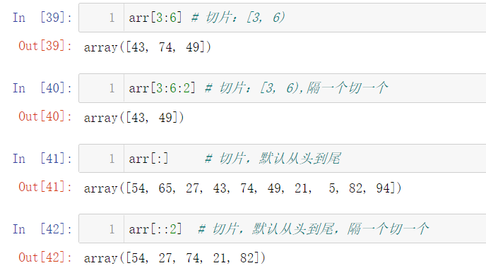
8.1 one dimensional array index and slicing

8.2 two dimensional array index and slicing

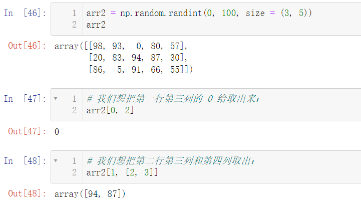
What should we do if we want to extract data with multiple rows and columns?

Obviously, the output result is not what we want to output. This is because if we want to take out multiple rows and columns, we need to use indexes and slices together:

You may be a little confused. It's okay. Let's give more examples:

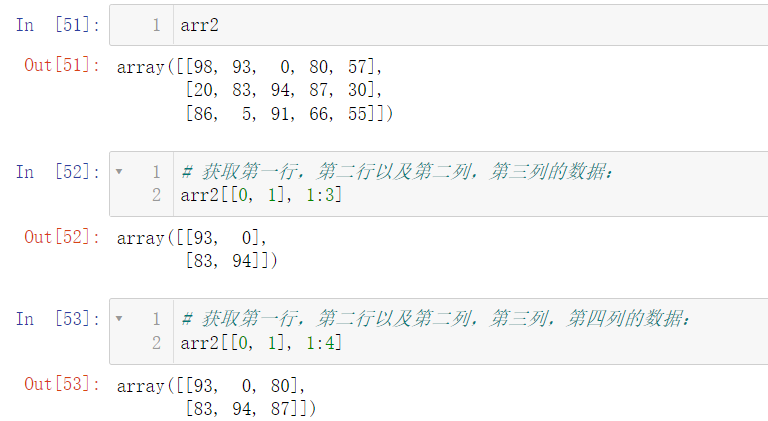
Let's look back and see what was taken out by the wrong operation just now:

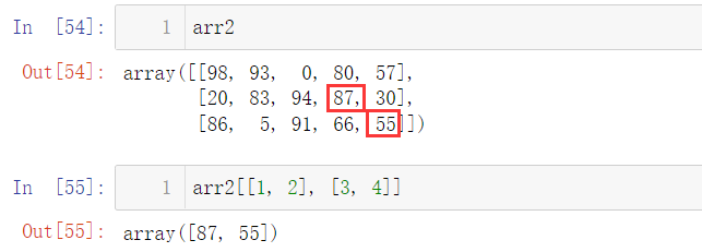
It is not difficult to see that we take the values of (1, 3) and (2, 4) positions

❗ Next, let's start the operation: if the rows and columns are not continuous, how to get them? For example, I want to take the number of the first row, the third row, the second column and the fourth column:

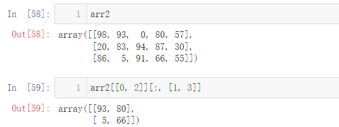
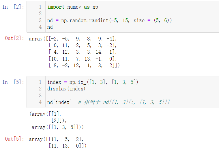
Next, another method is introduced, which can also be realized:

We can also change the value in the array. We just need to find the corresponding index:

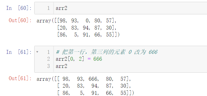
Of course, we can change multiple values at once:

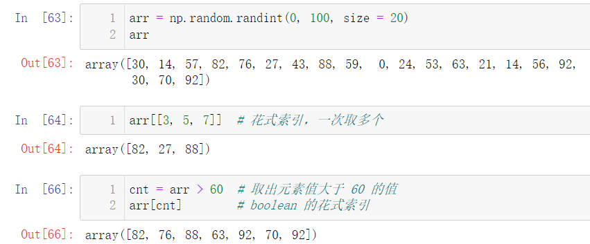
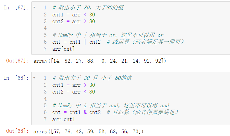
8.3 fancy index

The so-called fancy index is actually taking out multiple values at one time

9. Training ground

🚩 The training ground contains ten example questions and answer codes. Readers need to write them by themselves to enhance their learning and memory.

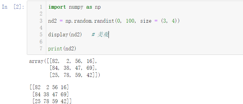
Here, I'd like to introduce a function: display(), which is similar to the print() function, but it is more beautiful than print:

9.1 create a one-dimensional all 0 ndarray object with a length of 10, and then make the fifth element equal to 1

# Create a one-dimensional all 0 ndarray object with a length of 10, and then make the fifth element equal to 1
import numpy as np
arr = np.zeros(10, dtype = 'int')

# 5th
arr[4] = 1
arr

9.2 create an ndarray object with elements from 10 to 49 with an interval of 1

# Create an ndarray object with elements from 10 to 49 (including 49), with an interval of 1
import numpy as np

# Note that it contains 49, so we need to pass it to 50 when giving the function string parameters
arr = np.arange(10, 50)
arr

9.3 reverse the position of all elements in question 2

# Reverse the positions of all elements in question 2
import numpy as np

# Note that it contains 49, so we need to pass it to 50 when giving the function string parameters
arr = np.arange(10, 50)
arr

# Elements can be flipped using the reverse slice operation
arr = arr[::-1]
arr

9.4 using NP random. Random creates a 10 * 10 ndarray object and prints out the largest and smallest elements

# Use NP random. Random creates a 10 * 10 ndarray object and prints out the largest and smallest elements
import numpy as np
arr = np.random.random(size = (10, 10))

# Use max and min to calculate the maximum and minimum elements respectively
print('The maximum value is:', arr.max())
print('The minimum value is:', arr.min())

9.5 create a 10 * 10 ndarray object, and the matrix boundary is all 1 and the inside is all 0

# Create a 10 * 10 ndarray object, and the matrix boundary is all 1 and the inside is all 0
import numpy as np
arr = np.full(shape = (10, 10), fill_value = 0, dtype = np.int8)

# The first and last lines are assigned a value of 1
arr[[0, -1]] = 1
# The first and last columns are assigned a value of 1
arr[:, [0, -1]] = 1

arr

9.6 create a 5 * 5 matrix with each row from 0 to 4

# Create a 5 * 5 matrix with each row from 0 to 4
import numpy as np

# First create a matrix with all elements of 0
arr = np.zeros((5, 5), dtype = int)

# Sequential addition
arr += np.arange(5)

arr

9.7 create an arithmetic sequence with a length of 12 between (0,1) and [1, 2, 4, 8, 16, 32, 64, 128, 256, 512, 1024] arithmetic sequence.

# Create an arithmetic sequence with a length of 12 in the range (0,1)
# Create [1, 2, 4, 8, 16, 32, 64, 128, 256, 512, 1024] proportional series
import numpy as np

# Arithmetic sequence
arr = np.linspace(0,1,12)
display(arr)

# Proportional sequence
arr2 = np.logspace(0, 10, base = 2, num = 11, dtype = int)
arr2

9.8 create a positive distribution array NP with a length of 10 random. Randn and sort

# Create a positive distribution array NP with a length of 10 random. Randn and sort
import numpy as np

# Create a random array
arr = np.random.randn(10)
print('Unsorted:', arr)

# Call NP The sort () method requires a new array to accept data
arr2 = np.sort(arr)
print('After sorting:', arr2)

9.9 create a random array with a length of 10 and replace the maximum value with - 100

# Create a random array with a maximum length of - 100
import numpy as np

# Scientific counting is not used
np.set_printoptions(suppress = True)

# Create random array
arr = np.random.random(10)
print('Original data:', arr)

# Maximum found
Max = arr.max()
# Make conditional judgment
cnt = arr == Max
# Change assignment
arr[cnt] = -100

# Output changed array
print('After change:', arr)

9.10 how to sort a 5 * 5 matrix according to the size order of column 3?

# How to sort a 5 * 5 matrix according to the size order of column 3? (argsort() method)
import numpy as np

# Let's explain the argsort() method first:
arr = np.random.randint(0, 100, size = 5)
display(arr)

# argsort() returns the sorted index subscript
index = np.argsort(arr)
display(index)

# Sort by index: fancy index
arr[index]

import numpy as np

# Return to the title requirements
arr = np.random.randint(0, 30, size = (5, 5))
display(arr)

# Gets the index order of the third column
index = arr[:, 2].argsort()

# The arr is sorted according to the index order of the third column
arr[index]

2, Numpy advanced

1. Data shape change

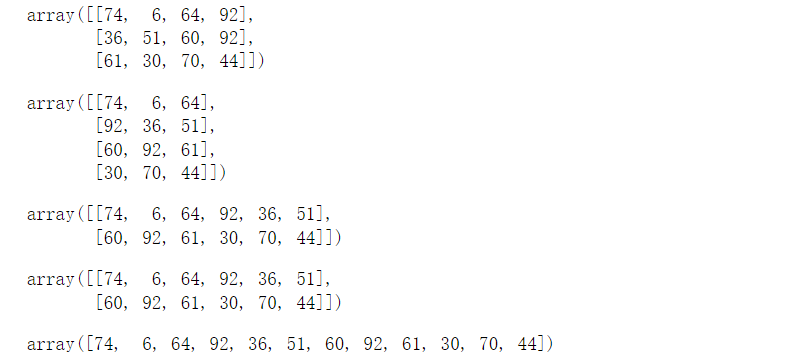
1.1 array deformation

🚩 We can use reshape() method to change the shape of the array arbitrarily:

import numpy as np

nd2 = np.random.randint(0, 100, size = (3, 4))

display(nd2)

# reshape data
# Our nd2 is an array of three rows and four columns. We can turn it into four rows and three columns
display(nd2.reshape(4, 3))

# For another example, let's turn it into two rows and six columns
# Method 1:
display(nd2.reshape(2, 6))
# Method 2:
display(nd2.reshape(-1, 6))
# -1 represents the final calculation: equivalent to X * 6 = 3 * 4 -- > x = 2
# -1. It is suitable for those who do not care about the total number and do not care about the total number. It is more flexible
display(nd2.reshape(-1))
# Equivalent to x = 3 * 4 -- > x = 12

1.2 array stacking

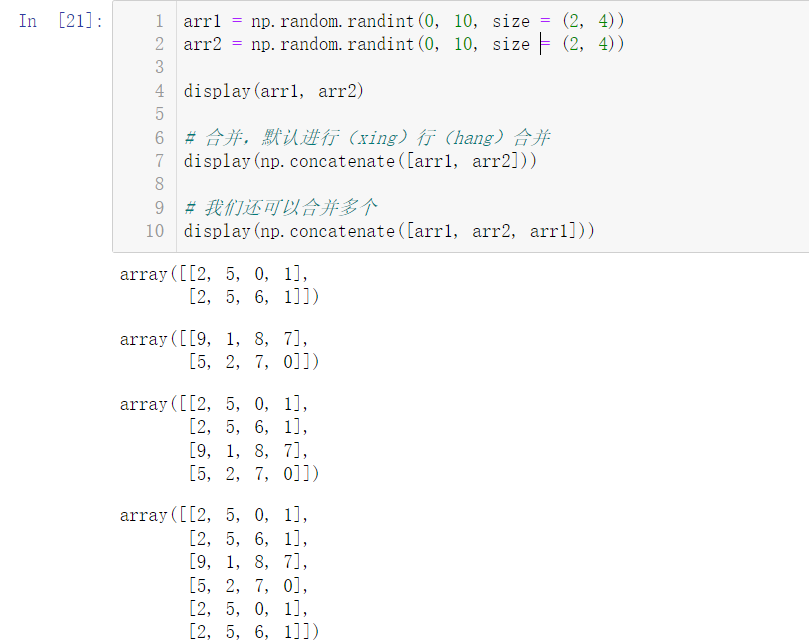
🚩 We can use concatenate() to merge arrays:

arr1 = np.random.randint(0, 10, size = (2, 4))
arr2 = np.random.randint(0, 10, size = (2, 4))

display(arr1, arr2)

# Merge: by default, a (xing) row (hang) merge is performed
display(np.concatenate([arr1, arr2]))

# We can also merge multiple
display(np.concatenate([arr1, arr2, arr1]))

So can we combine an array of three rows and four columns with an array of four rows and three columns?

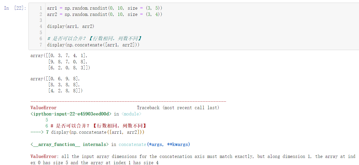
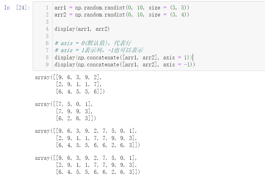
Is there really no way? In fact, it is not. By observing the two arrays, we can find that although the number of columns of the two arrays is different, the number of rows of the two arrays is the same, so we can merge columns:

arr1 = np.random.randint(0, 10, size = (3, 5))
arr2 = np.random.randint(0, 10, size = (3, 4))

display(arr1, arr2)

# Axis = 0 (default), representing the row
# axis = 1 represents a column, - 1 can also represent a column
display(np.concatenate([arr1, arr2], axis = 1))
display(np.concatenate([arr1, arr2], axis = -1))

1.3 array splitting

🚩 Use the split() function to split the array:

nd = np.random.randint(0, 100, size = (6, 9))

display(nd)

# Row split
display(np.split(nd, 2)) # Split into 2 parts on average
display(np.split(nd, 3)) # Split into 3 parts on average

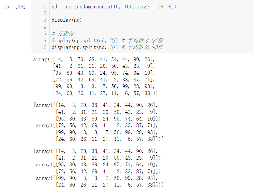
We can also not split equally:

nd = np.random.randint(0, 100, size = (6, 9))

display(nd)

# The list represents splitting by node
np.split(nd, [1, 4, 5])
# 1 cut, 4 cut, 5 cut
# Divided into [0, 1) [1, 4) [4, 5) [5, 6)

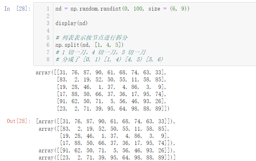
We can split not only rows, but also columns. Just like 2.1.2 array stacking, the parameter axis = 0 (default value) represents rows and axis = 1 represents columns

nd = np.random.randint(0, 100, size = (6, 9))

display(nd)

np.split(nd, 3, axis = 1) # Average split into three parts (column split)
# The list represents splitting by node
np.split(nd, [1, 4, 5], axis = 1)
# 1 cut, 4 cut, 5 cut
# Divided into [0, 1) [1, 4) [4, 5) [5, 9)

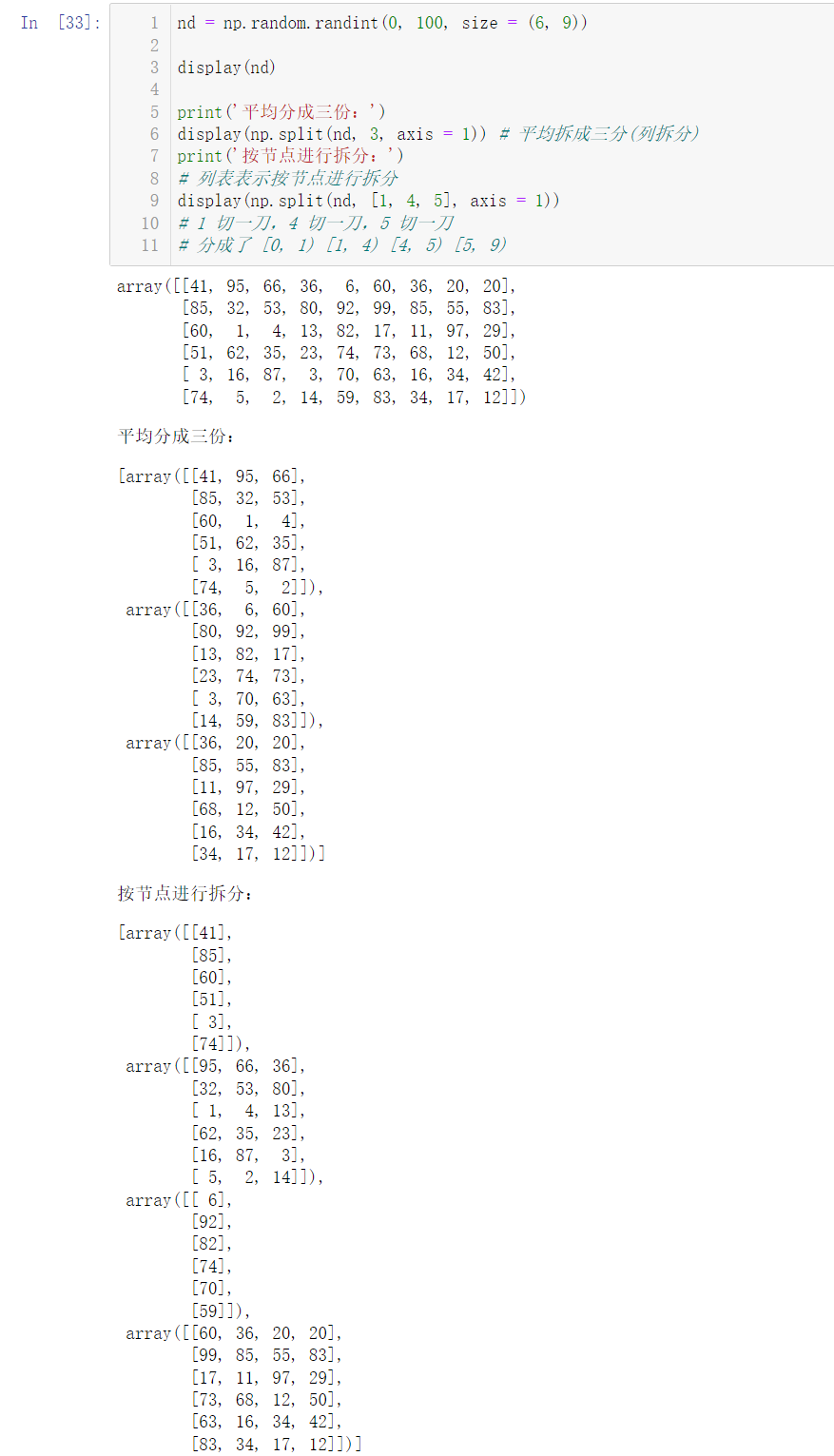
1.4 array transpose

🚩 For the transpose of arrays, we can use T to transpose, or use the transfer() method in numpy:

A = np.random.randint(0, 10, size = (3, 5))

display(A)

# The so-called transpose is that rows change into columns, and columns edge rows
display(A.T)
# You can also transpose according to the following method
display(np.transpose(A, axes = [1, 0]))

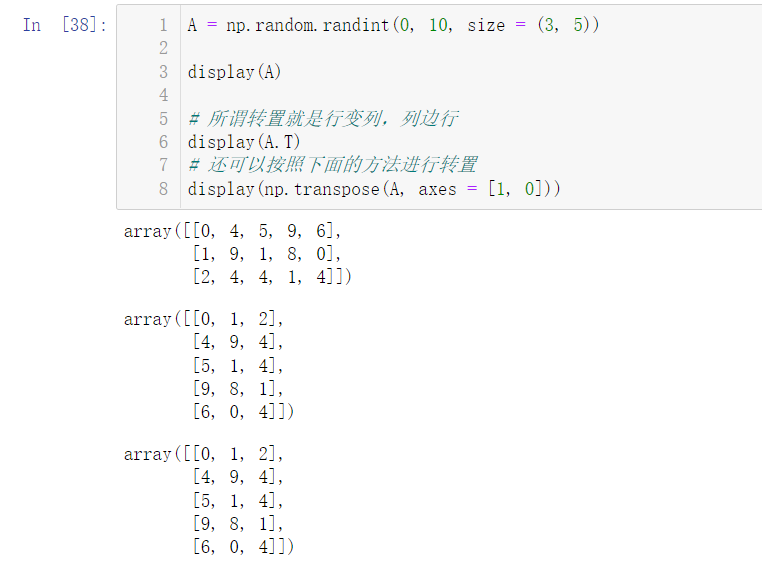
2. Broadcasting mechanism

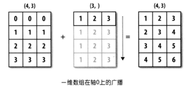
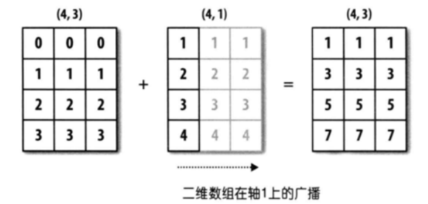
🚩 The so-called broadcast is to continuously copy the original data to the same structure as the target array. For example, if we have an array with three rows and four columns, we need to add an array with one row and four columns, then the array with one row and four columns will copy three copies to become an array with three rows and four columns, in which each row has the same value as the original array. After this form, Then add with the original array of three rows and four columns. Next, we demonstrate the code from three aspects: broadcasting of one-dimensional array, broadcasting of two-dimensional array and broadcasting of three-dimensional array.

2.1 broadcasting of one-dimensional array

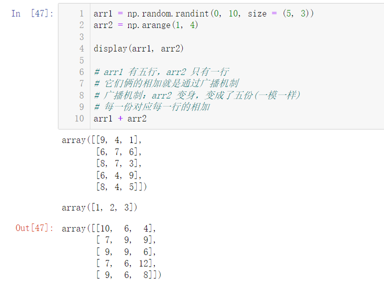
arr1 = np.random.randint(0, 10, size = (5, 3))
arr2 = np.arange(1, 4)

display(arr1, arr2)

# arr1 has five lines and arr2 has only one line
# They add up through the broadcast mechanism
# Broadcasting mechanism: arr2 as like as two peas, five copies.
# Each copy corresponds to the addition of each line
arr1 + arr2

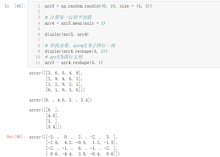
2.2 broadcasting of two-dimensional array

arr3 = np.random.randint(0, 10, size = (4, 5))

# Calculate the average value of each row
arr4 = arr3.mean(axis = 1)

display(arr3, arr4)

# Note that there are 5 numbers in each row of arr3 and 4 numbers in each row of arr4
arr3 - arr4 # The shape does not match, so an error is reported

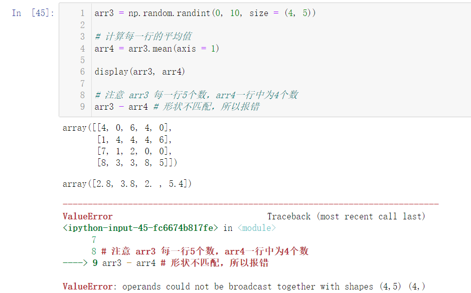
An error will be reported because the shapes do not match. We can use the reshape() method in 2.1.1 array deformation to change the array:

arr3 = np.random.randint(0, 10, size = (4, 5))

# Calculate the average value of each row
arr4 = arr3.mean(axis = 1)

display(arr3, arr4)

# The shape is changed, and arr4 is changed to four rows and one column
display(arr4.reshape(4, 1))
# arr3 is four rows and five columns
arr3 - arr4.reshape(4, 1)

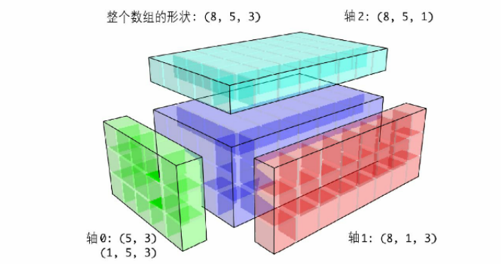
2.3 broadcasting of 3D array

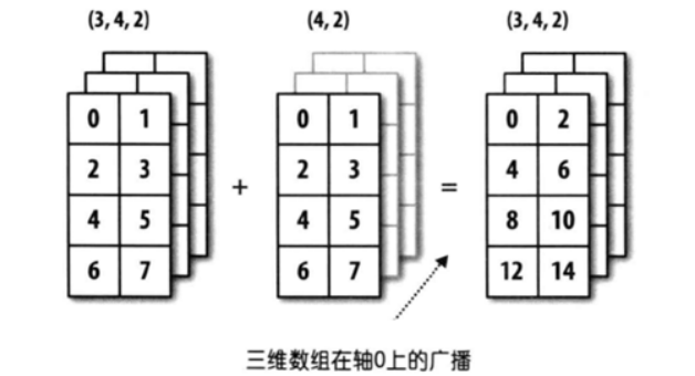
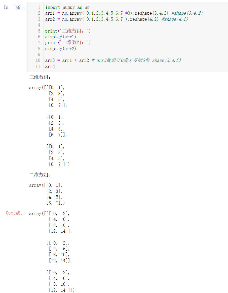
import numpy as np 
arr1 = np.array([0,1,2,3,4,5,6,7]*3).reshape(3,4,2) #shape(3,4,2) 
arr2 = np.array([0,1,2,3,4,5,6,7]).reshape(4,2) #shape(4,2) 

print('3D array:')
display(arr1)
print('2D array:')
display(arr2)

arr3 = arr1 + arr2 # The arr2 array copies three shapes (3,4,2) in the 0 dimension 
arr3

3. General function

3.1 element level digital functions

🚩 NumPy has many math related functions: abs, sqrt, square, exp, log, sin, cos, tan, maximum, minimum, all, any, inner, clip, round, trace, ceil, floor. Let's select some commonly used functions for code demonstration. Interested readers can search for the usage of other functions and practice them by themselves. We won't do too much demonstration here:

# PI
display(np.pi)

# Calculated sin90 °
display(np.sin(90))  # This is illegal. 90 is an int, not a degree
display(np.sin(np.pi / 2))  # PI is 180 °, so pi / 2 stands for 90 °

# Calculate cos90 °
display(np.cos(np.pi / 2))

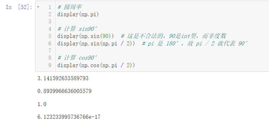
An interesting phenomenon appears. The result of calculating cos 90 ° does not display 0, but e-7. This is because we will have accuracy problems in the calculation process, so we generally represent 0, that is, when a number is less than a small number, we think the number is 0. We can use the round(n) function to keep N decimal places:

# Keep one decimal place:
display(np.cos(np.pi / 2).round(1))
# Keep five decimal places:
display(np.cos(np.pi / 2).round(5))

It can be seen that even if we keep five decimal places, it is still 0, so we think this number is 0

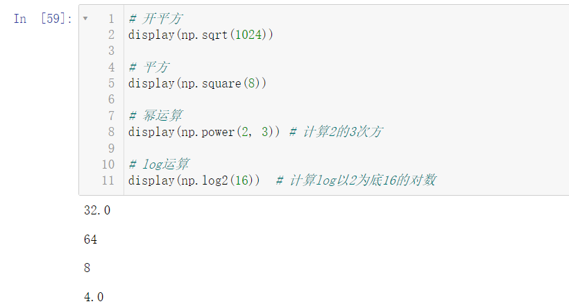
# Open square
display(np.sqrt(1024))

# square
display(np.square(8))

# exponentiation 
display(np.power(2, 3)) # Calculate the third power of 2

# log operation
display(np.log2(16))  # Calculate the logarithm of log base 16 of 2

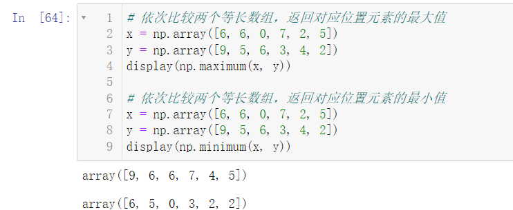
# Compare two equal length arrays in turn and return the maximum value of the corresponding position element
x = np.array([6, 6, 0, 7, 2, 5]) 
y = np.array([9, 5, 6, 3, 4, 2]) 
display(np.maximum(x, y))

# Compare two equal length arrays in turn and return the minimum value of the corresponding position element
x = np.array([6, 6, 0, 7, 2, 5]) 
y = np.array([9, 5, 6, 3, 4, 2])
display(np.minimum(x, y))

# Returns the inner product of a one-dimensional array vector
arr = np.random.randint(0, 10, size = (2, 2)) 
display(arr)
np.inner(arr[0], arr)

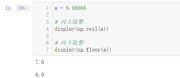
a = 6.66666

# Round up
display(np.ceil(a))

# Round down
display(np.floor(a))

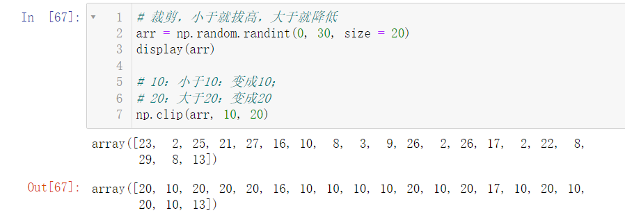
# Cut. If it is less than, it will be raised, and if it is greater than, it will be lowered
arr = np.random.randint(0, 30, size = 20)
display(arr)

# 10: Less than 10: becomes 10;
# 20: Greater than 20: becomes 20
np.clip(arr, 10, 20)

3.2 where function

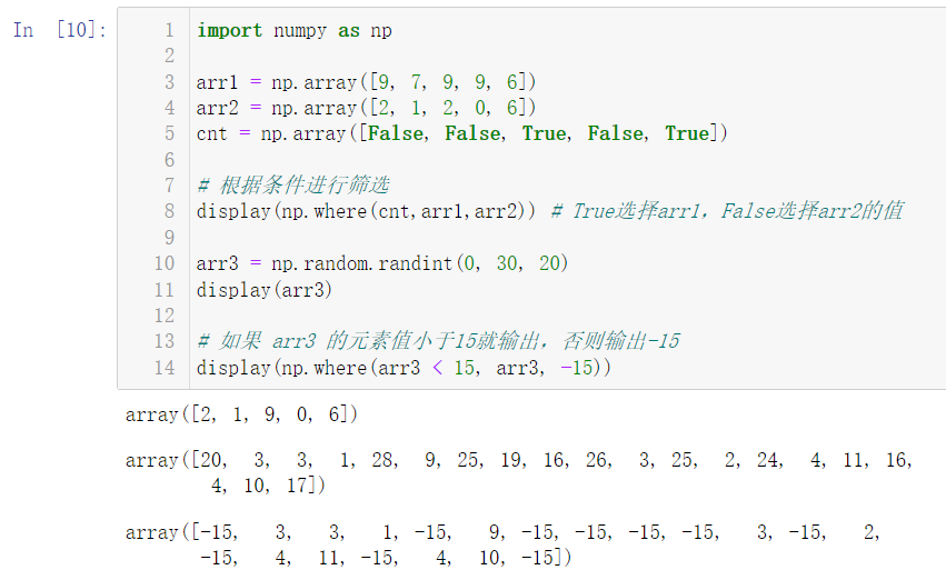
import numpy as np 

arr1 = np.array([9, 7, 9, 9, 6]) 
arr2 = np.array([2, 1, 2, 0, 6]) 
cnt = np.array([False, False, True, False, True]) 

# Filter by criteria
display(np.where(cnt,arr1,arr2)) # True selects arr1 and False selects the value of arr2

arr3 = np.random.randint(0, 30, 20)
display(arr3)

# If the element value of arr3 is less than 15, it will be output, otherwise - 15 will be output
display(np.where(arr3 < 15, arr3, -15))

3.3 sorting method

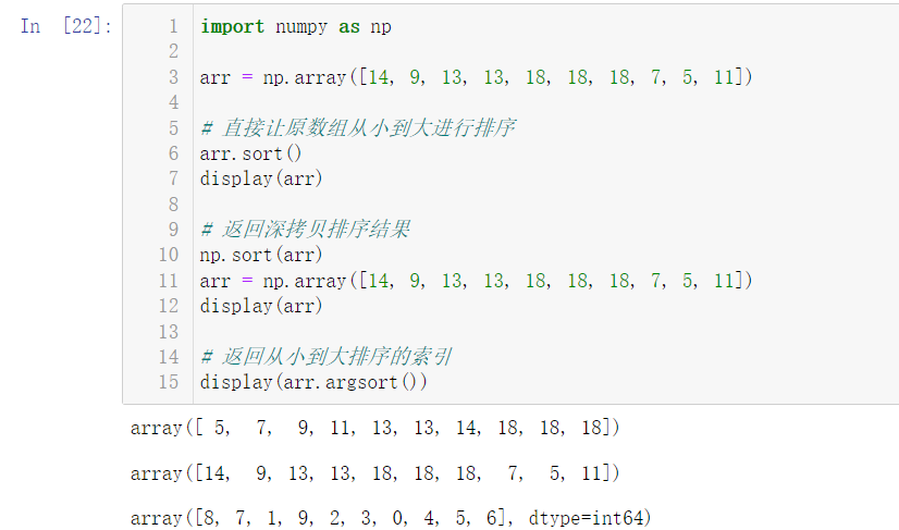
🚩 NumPy also provides sorting methods. The sorting method is local sorting, that is, directly changing the original array:
arr.sort(),np.sort(),arr.argsort()

import numpy as np 

arr = np.array([14, 9, 13, 13, 18, 18, 18, 7, 5, 11]) 

# Directly sort the original array from small to large
arr.sort() 
display(arr)

# Returns the deep copy sort result 
np.sort(arr)
arr = np.array([14, 9, 13, 13, 18, 18, 18, 7, 5, 11]) 
display(arr)

# Returns the index sorted from small to large
display(arr.argsort()) 

3.4 set operation function

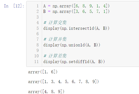
A = np.array([6, 8, 9, 1, 4])
B = np.array([3, 6, 5, 7, 1]) 

# Calculate intersection
display(np.intersect1d(A, B))

# Computational Union
display(np.union1d(A, B))

# Computational difference set
display(np.setdiff1d(A, B))

3.5 mathematical and statistical functions

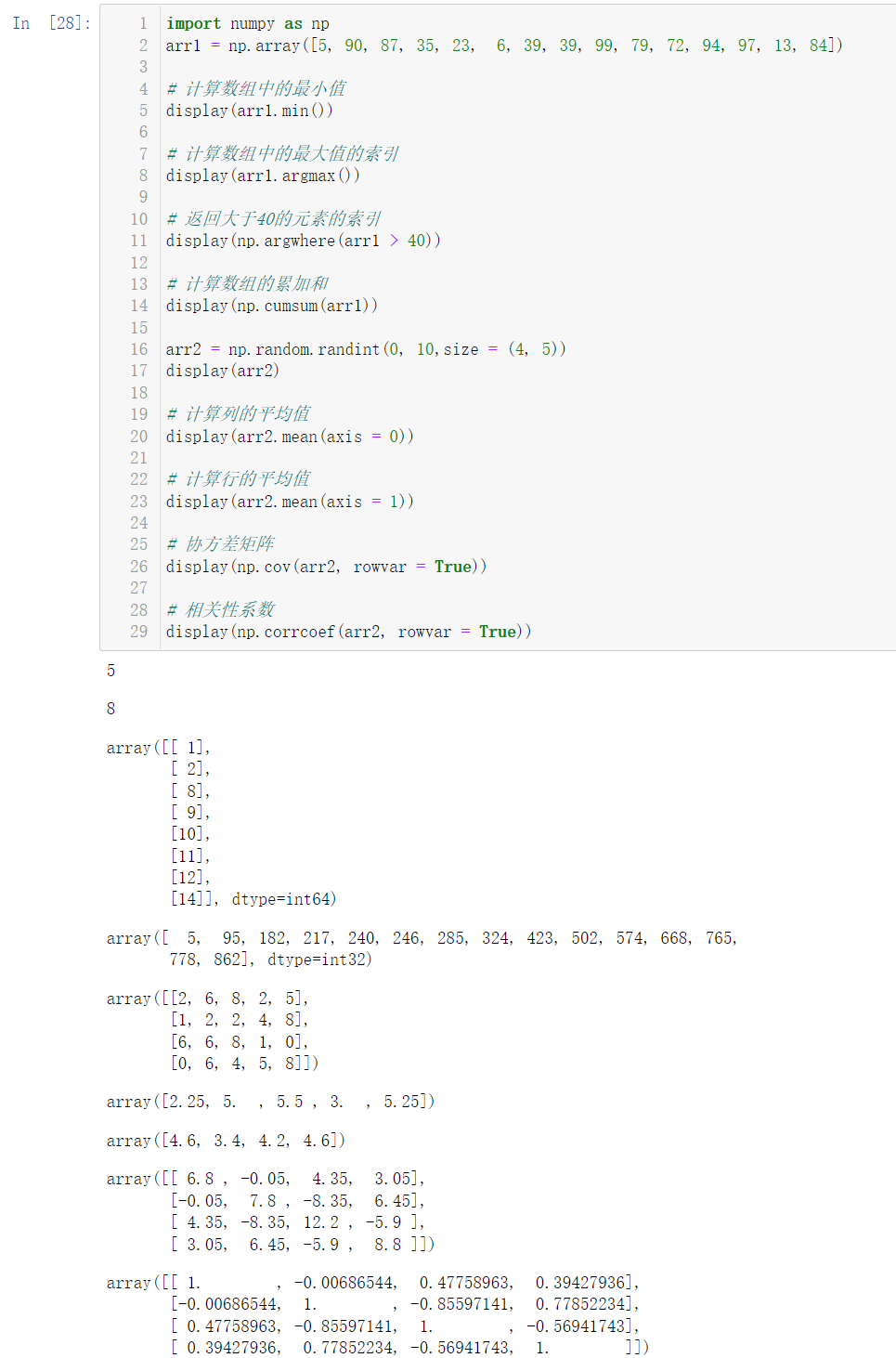
🚩 We select several commonly used functions for code demonstration, and interested readers of the remaining functions can refer to the usage and demonstration by themselves. min,max,mean,median,sum,std,var,cumsum,cumprod,argmin,argmax,argwhere,cov,corrcoef

import numpy as np 
arr1 = np.array([5, 90, 87, 35, 23,  6, 39, 39, 99, 79, 72, 94, 97, 13, 84]) 

# Calculates the minimum value in the array
display(arr1.min())

# The maximum calculated value in the index array
display(arr1.argmax())

# Returns the index of an element greater than 40
display(np.argwhere(arr1 > 40))

# Calculate the cumulative sum of the array
display(np.cumsum(arr1))

arr2 = np.random.randint(0, 10,size = (4, 5))
display(arr2)

# Calculate the average of the columns
display(arr2.mean(axis = 0))

# Calculate the average of rows
display(arr2.mean(axis = 1))

# covariance matrix 
display(np.cov(arr2, rowvar = True))

# Correlation coefficient
display(np.corrcoef(arr2, rowvar = True))

4. Matrix operation

4.1 matrix multiplication

#Product of matrix (point multiplication)
A = np.array([[2, 1, 7], 
              [6, 3, 4]]) # shape(2, 3) 
B = np.array([[4, 3], 
              [0, 9], 
              [-5, -8]]) # shape(3, 2) 
# The first method 
display(np.dot(A,B))
# The second method
display(A @ B) # The symbol @ denotes the matrix product operation
# The third method
display(A.dot(B))

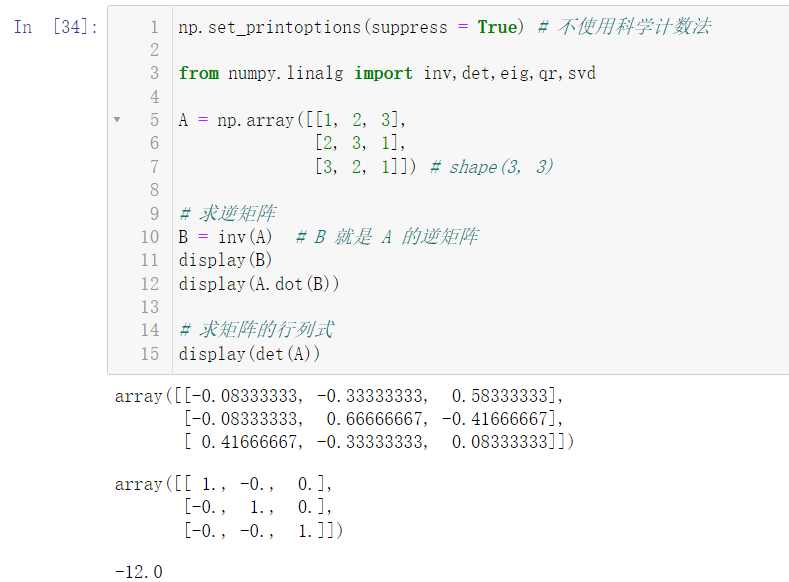
4.2 other operations of matrix

np.set_printoptions(suppress = True) # Scientific counting is not used

from numpy.linalg import inv,det,eig,qr,svd 

A = np.array([[1, 2, 3], 
              [2, 3, 1], 
              [3, 2, 1]]) # shape(3, 3) 

# Inverse matrix
B = inv(A)  # B is the inverse of A
display(B)
display(A.dot(B))

# Find determinant of matrix
display(det(A))

5. Training ground

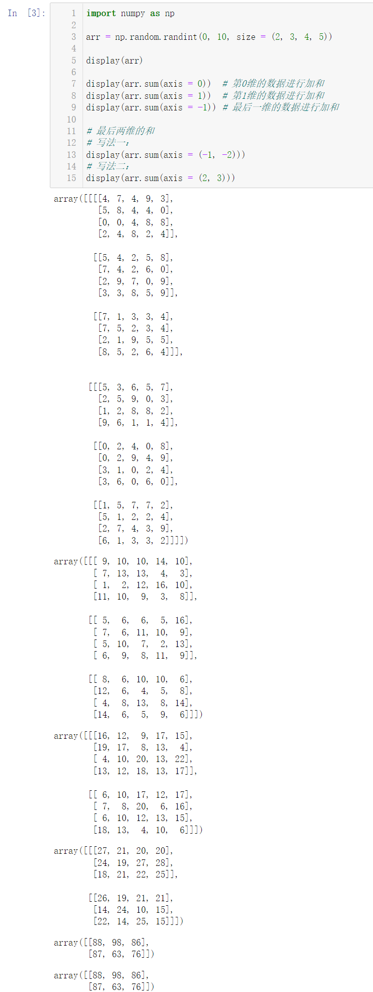
5.1 given a 4-dimensional matrix, how to get the sum of the last two dimensions? (prompt, specify axis for calculation)

import numpy as np

arr = np.random.randint(0, 10, size = (2, 3, 4, 5))

display(arr)

display(arr.sum(axis = 0))  # Add the data of dimension 0
display(arr.sum(axis = 1))  # Add the data in the first dimension
display(arr.sum(axis = -1)) # Finally, one-dimensional data are added

# Sum of the last two dimensions
# Writing method 1:
display(arr.sum(axis = (-1, -2)))
# Method 2:
display(arr.sum(axis = (2, 3)))

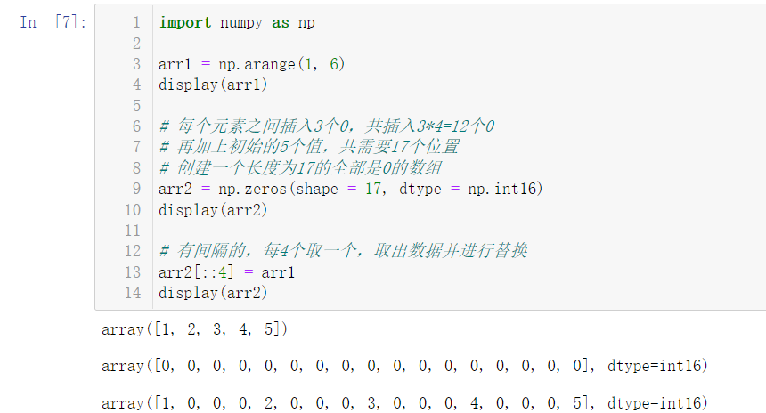
5.2 given an array [1, 2, 3, 4, 5], how to get a new array after inserting 3 zeros between each element of this array?

import numpy as np

arr1 = np.arange(1, 6)
display(arr1)

# Insert 3 zeros between each element, and a total of 3 * 4 = 12 zeros are inserted
# Plus the initial 5 values, a total of 17 positions are required
# Create an array of all zeros with a length of 17
arr2 = np.zeros(shape = 17, dtype = np.int16)
display(arr2)

# If there are intervals, take one every four, take out the data and replace it
arr2[::4] = arr1
display(arr2)

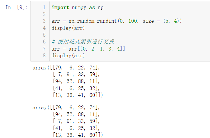
5.3 given a two-dimensional matrix (5 rows and 4 columns), how to exchange the elements of two rows (prompt: arbitrary adjustment, fancy index)?

import numpy as np

arr = np.random.randint(0, 100, size = (5, 4))
display(arr)

# Swap using fancy indexes
arr = arr[[0, 2, 1, 3, 4]]
display(arr)

5.4 create a random array with length of 100000, use two methods to find the third power (1. for loop; 2. NumPy's own method), and compare the time used

%%Time: it can display the running time of the code, which will be linked to the performance of the computer
Using the for loop

%%time
import numpy as np

arr = np.random.randint(0, 10, size = 100000)
res = []

for item in arr:
    res.append(item ** 3)

Use NumPy's own method

%%time
import numpy as np

arr = np.random.randint(0, 10, size = 100000)
res = []

arr2 = np.power(arr, 3)

It can be found that using the built-in method of NumPy is much more efficient than using the for loop

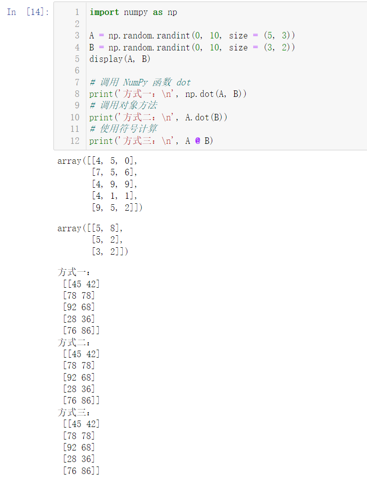
5.5 create a random matrix with 5 rows and 3 columns and a random matrix with 3 rows and 2 columns to calculate the matrix product

import numpy as np

A = np.random.randint(0, 10, size = (5, 3))
B = np.random.randint(0, 10, size = (3, 2))
display(A, B)

# Call NumPy function dot
print('Mode 1:\n', np.dot(A, B))
# Call object method
print('Mode 2:\n', A.dot(B))
# Calculate using symbols
print('Mode 3:\n', A @ B)

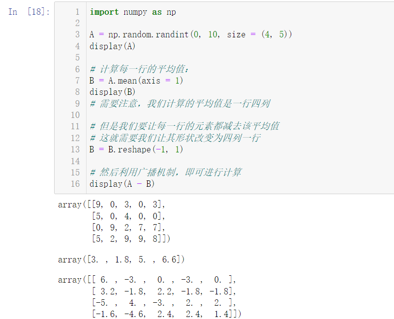
5.6 the elements of each row of the matrix subtract the average value of the row (note that axis is specified when calculating the average value, and the shape changes during subtraction)

import numpy as np

A = np.random.randint(0, 10, size = (4, 5))
display(A)

# Calculate the average value of each row:
B = A.mean(axis = 1)
display(B)
# Note that the average value we calculated is one row and four columns

# But let's subtract the average from the elements of each row
# This requires us to change its shape to four columns and one row
B = B.reshape(-1, 1) 

# Then, the broadcast mechanism can be used for calculation
display(A - B)

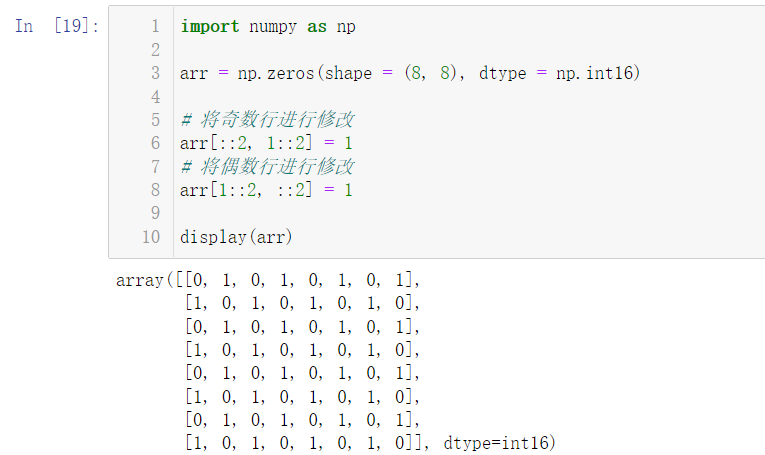
5.7 print out the following functions (np.zeros is required to create an 8 * 8 matrix):

[[0 1 0 1 0 1 0 1]
[1 0 1 0 1 0 1 0]
[0 1 0 1 0 1 0 1]
[1 0 1 0 1 0 1 0]
[0 1 0 1 0 1 0 1]
[1 0 1 0 1 0 1 0]
[0 1 0 1 0 1 0 1]
[1 0 1 0 1 0 1 0]]

import numpy as np

arr = np.zeros(shape = (8, 8), dtype = np.int16)

# Modify odd rows
arr[::2, 1::2] = 1
# Modify even rows
arr[1::2, ::2] = 1

display(arr)

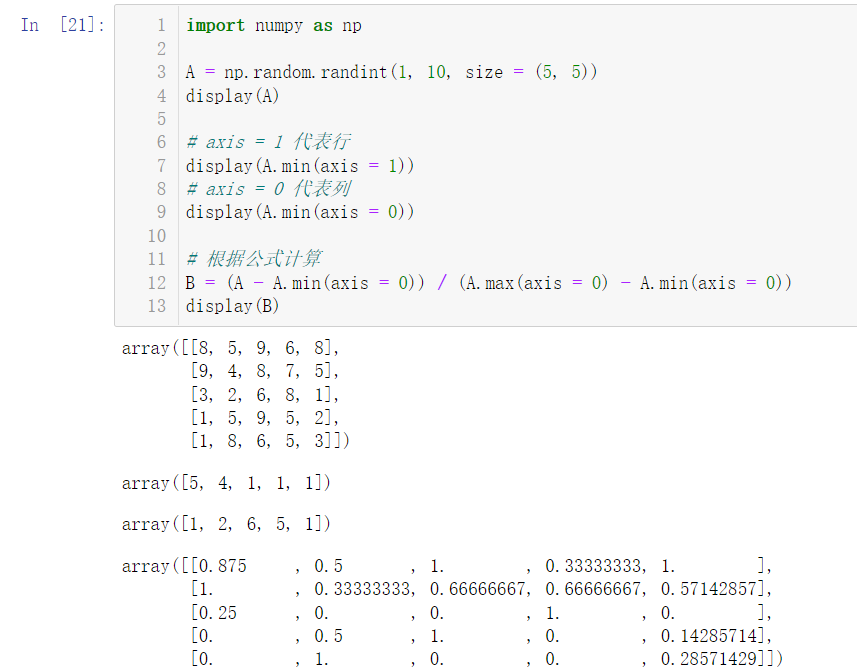
5.8 regularize a random matrix with 5 rows and 5 columns (the data is uniformly changed into a number between 0 and 1, which is equivalent to reduction)

Concept of regularity: subtract the minimum value of each column in matrix A, divide by the maximum value of each column, and subtract the minimum value of each column (prompt:
axis give appropriate parameters!!!)

A = A − A . m i n A . m a x − A . m i n \rm{A = \frac{A - A.min}{A.max - A.min}} A=A.max−A.minA−A.min​

import numpy as np

A = np.random.randint(1, 10, size = (5, 5))
display(A)

# axis = 1 represents the row
display(A.min(axis = 1))
# axis = 0 represents the column
display(A.min(axis = 0))

# Calculated according to the formula
B = (A - A.min(axis = 0)) / (A.max(axis = 0) - A.min(axis = 0))
display(B)

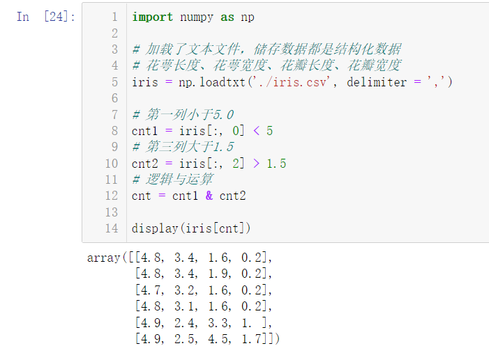
5.9 how to filter numpy arrays according to two or more conditions. Load iris data, and filter the data according to the condition that the first column is less than 5.0 and the third column is greater than 1.5. (hint, you need to use logical and operation: &)

Our data:

Link: https://pan.baidu.com/s/1VaPHJa6YttfnedO0ewDRtQ
Extraction code: 5u92

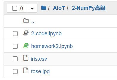
After downloading the data, we move it to the following folder: (download it directly to the desktop, find the location of the folder, and then drag it in)


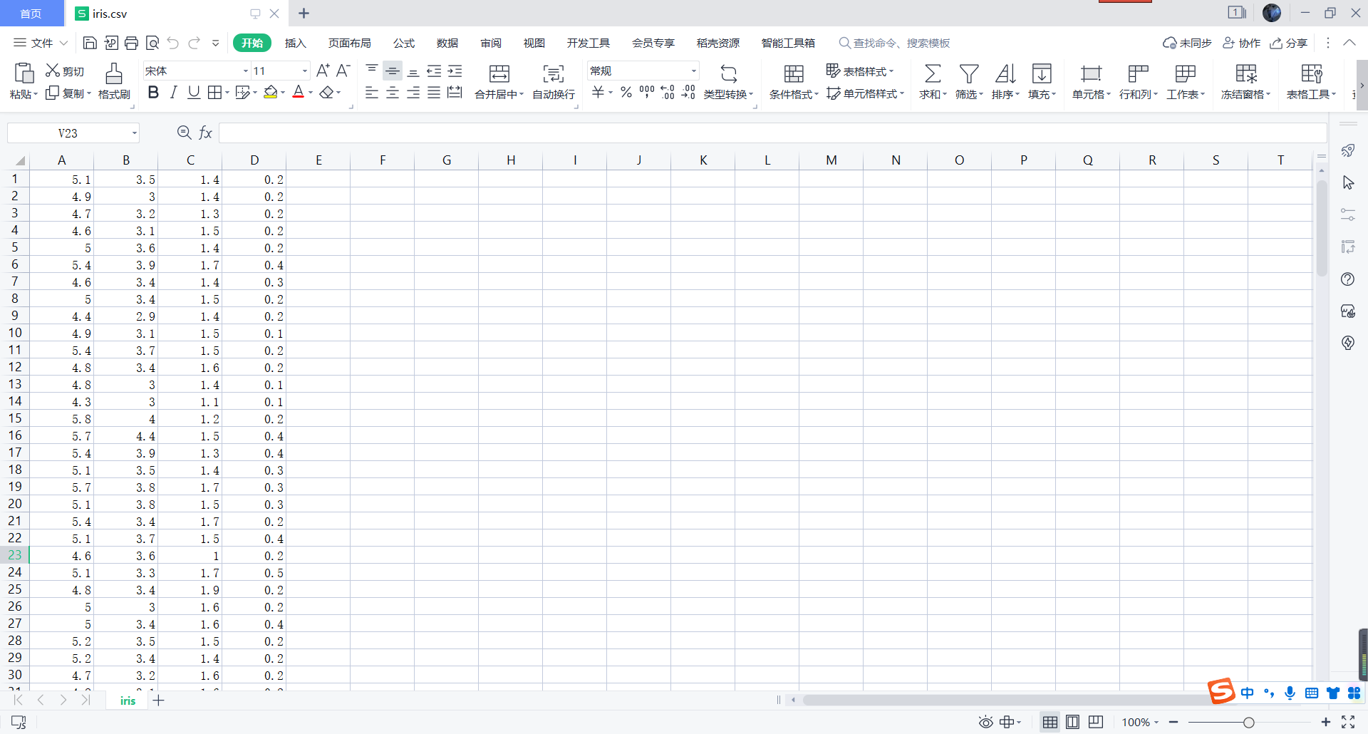
First, let's introduce it csv file, which is actually a text file. We open it (the default opening path is Excel)

We can also choose to open it in Notepad mode:

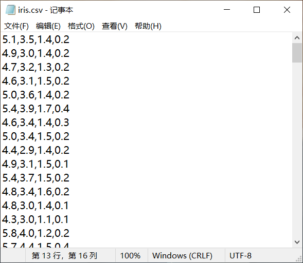
Through observation, it is not difficult to see that the data are separated

Next, we introduce a new method: loadtext (), which is used to load data, such as NP Loadtext ('. / iris.csv', delimiter = '' '), which is used to open the path'/ iris.csv 'files. These data are separated directly through.

import numpy as np

# Loaded text files, stored data are structured data
iris = np.loadtxt('./iris.csv', delimiter = ',')

display(iris)

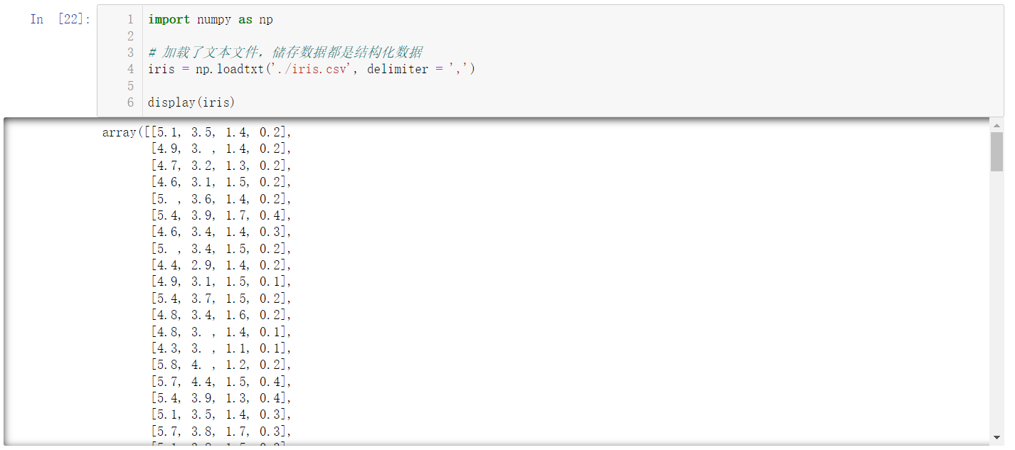
It can be seen that these data are expanded in the form of two-dimensional arrays, and there are four data in each dimension, representing calyx length, calyx width, petal length and petal width respectively

import numpy as np

# Loaded text files, stored data are structured data
# Calyx length, calyx width, petal length, petal width
iris = np.loadtxt('./iris.csv', delimiter = ',')

# The first column is less than 5.0
cnt1 = iris[:, 0] < 5
# The third column is greater than 1.5
cnt2 = iris[:, 2] > 1.5
# Logic and operation
cnt = cnt1 & cnt2

display(iris[cnt])

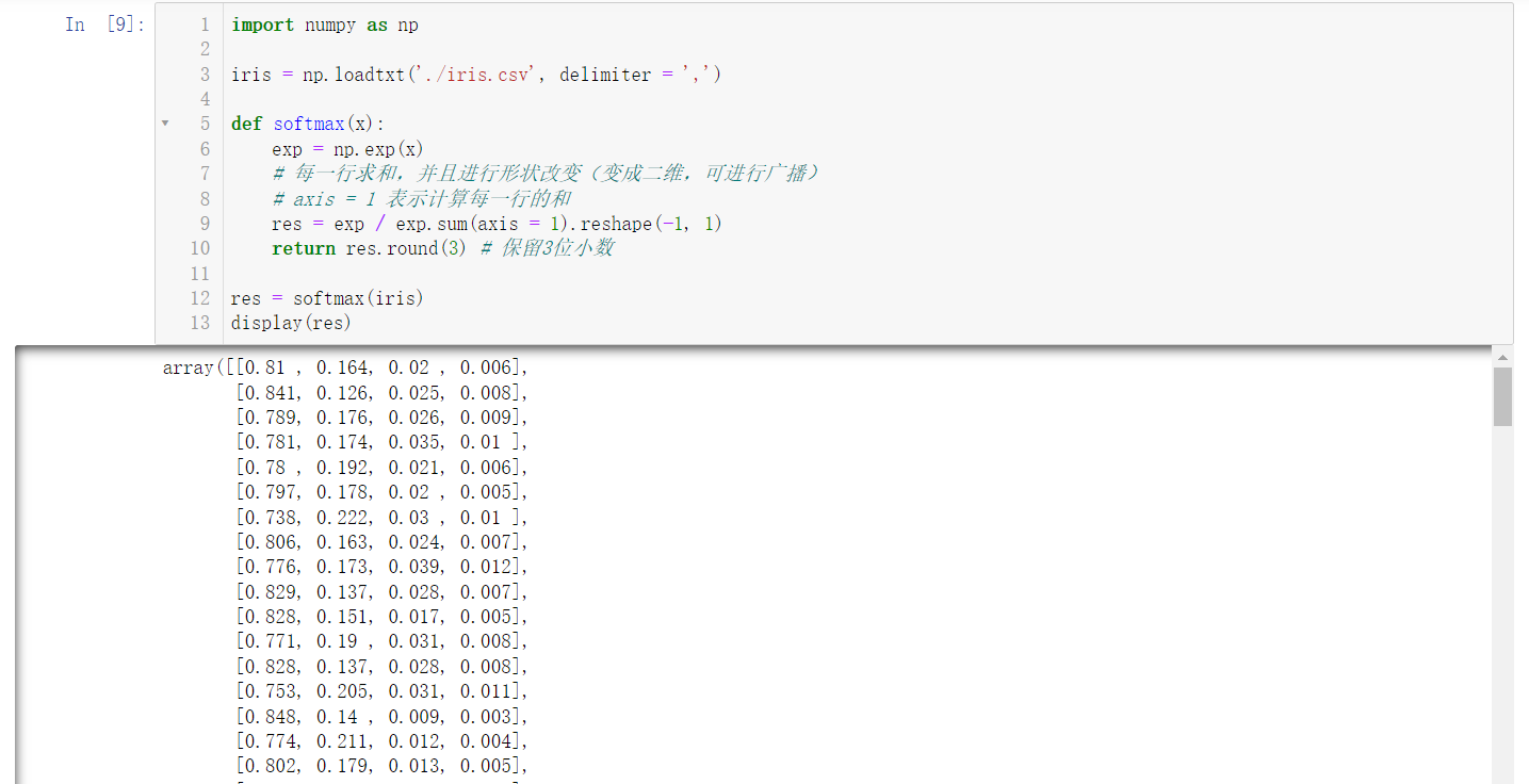
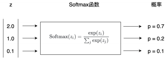
5.10 calculate the softmax score of each row of iris data (exp represents the power operation of natural base e)

import numpy as np

iris = np.loadtxt('./iris.csv', delimiter = ',')

def softmax(x):
    exp = np.exp(x)
    # Sum each line and change the shape (become two-dimensional and broadcast)
    # axis = 1 means the sum of each row is calculated
    res = exp / exp.sum(axis = 1).reshape(-1, 1)
    return res.round(3) # Keep 3 decimal places

res = softmax(iris)
display(res)