Original text: https://numpy.org/devdocs/user/quickstart.html
NumPy quick start
precondition
You need to know a little about Python. For review, see Python tutorial.
To run these examples, you need to install matplotlib in addition to NumPy.
brief introduction
This is a quick overview of arrays in NumPy. It demonstrates that n-dimensional (n > = 2) arrays are represented and can be manipulated. In particular, if you don't know how to apply common functions to n-dimensional arrays (without using a for loop), or if you want to understand the axis and shape properties of n-dimensional arrays, this article may be helpful.
Learning objectives
After reading, you should be able to:
- Understand the difference between one-dimensional, two-dimensional and n-dimensional arrays in NumPy;
- Learn how to apply some linear algebraic operations to n-dimensional arrays without using the for loop;
- Understand the axis and shape properties of n-dimensional arrays.
Basic knowledge
The main object of NumPy is an isomorphic multidimensional array. It is a table of elements (usually numbers), all of the same type, indexed by non negative integer tuples. In NumPy, dimensions are called axes.
For example, the coordinates [1, 2, 1] of a point in 3D space have only one axis. The axis has three elements, so we say its length is 3. In the example in the following figure, the array has 2 axes. The length of the first axis is 2 and the length of the second axis is 3.
[[1., 0., 0.],
 [0., 1., 2.]]
NumPy's array class is called ndarray. It is also called the alias array. Note that NumPy Array this is different from the standard Python library class Array, which handles only one-dimensional arrays and provides less functionality. The more important properties of the ndarray object are:
-
ndarray.ndim
The number of axes (dimensions) of the array.
-
ndarray.shape
The dimension of the array. This is an integer tuple indicating the size of the array in each dimension. For matrices with n rows and m columns, shape will be (n,m). The length of the shape tuple is the number of ndim axes,.
-
ndarray.size
The total number of elements in the array. This is equal to the product of the shape's elements.
-
ndarray.dtype
An object that describes the type of element in an array. You can create or specify dtype s using standard Python types. In addition, NumPy provides its own type. For example: NumPy int32,numpy.int16 and NumPy float64 .
-
ndarray.itemsize
The size (in bytes) of each element of the array. For example, an array itemsize of a float64 type element is 8 (= 64 / 8) and an element itemsize of a complex32 type is 4 (= 32 / 8). It is equivalent to darray.dtype.itemsize.
-
ndarray.data
Buffer containing the actual elements of the array. Generally, we don't need to use this attribute because we will use the indexing tool to access the elements in the array.
An example
>>> import numpy as np
>>> a = np.arange(15).reshape(3, 5)
>>> a
array([[ 0,  1,  2,  3,  4],
       [ 5,  6,  7,  8,  9],
       [10, 11, 12, 13, 14]])
>>> a.shape
(3, 5)
>>> a.ndim
2
>>> a.dtype.name
'int64'
>>> a.itemsize
8
>>> a.size
15
>>> type(a)
<class 'numpy.ndarray'>
>>> b = np.array([6, 7, 8])
>>> b
array([6, 7, 8])
>>> type(b)
<class 'numpy.ndarray'>
Array creation
There are several ways to create arrays.
For example, you can use the array function to create an array from a regular Python list or tuple. The type of the resulting array is derived from the type of the element in the sequence.
>>> import numpy as np
>>> a = np.array([2, 3, 4])
>>> a
array([2, 3, 4])
>>> a.dtype
dtype('int64')
>>> b = np.array([1.2, 3.5, 5.1])
>>> b.dtype
dtype('float64')
A common mistake is that array uses multiple parameter calls instead of providing a single sequence as a parameter.
>>> a = np.array(1, 2, 3, 4)    # WRONG
Traceback (most recent call last):
  ...
TypeError: array() takes from 1 to 2 positional arguments but 4 were given
>>> a = np.array([1, 2, 3, 4])  # RIGHT
Array converts a sequence into a two-dimensional array, a sequence into a three-dimensional array, and so on.
>>> b = np.array([(1.5, 2, 3), (4, 5, 6)])
>>> b
array([[1.5, 2. , 3. ],
       [4. , 5. , 6. ]])
The type of array can also be explicitly specified at creation:
>>> c = np.array([[1, 2], [3, 4]], dtype=complex)
>>> c
array([[1.+0.j, 2.+0.j],
       [3.+0.j, 4.+0.j]])
Usually, the elements of an array are initially unknown, but their size is known. Therefore, NumPy provides several functions to create an array with initial placeholder content. These minimize the additional operations required to grow the array.
The function zeros creates an all zero array, the function ones creates an all one array, and the function empty creates an array whose initial content is random and depends on the memory state. By default, the dtype of the created array is float64, but you can specify the dtype through the keyword parameter.
>>> np.zeros((3, 4))
array([[0., 0., 0., 0.],
       [0., 0., 0., 0.],
       [0., 0., 0., 0.]])
>>> np.ones((2, 3, 4), dtype=np.int16)
array([[[1, 1, 1, 1],
        [1, 1, 1, 1],
        [1, 1, 1, 1]],

       [[1, 1, 1, 1],
        [1, 1, 1, 1],
        [1, 1, 1, 1]]], dtype=int16)
>>> np.empty((2, 3))
array([[3.73603959e-262, 6.02658058e-154, 6.55490914e-260],  # may vary
       [5.30498948e-313, 3.14673309e-307, 1.00000000e+000]])
To create a sequence of numbers, NumPy provides range, which is similar to Python's built-in function range, but returns an array.
>>> np.arange(10, 30, 5)
array([10, 15, 20, 25])
>>> np.arange(0, 2, 0.3)  # it accepts float arguments
array([0. , 0.3, 0.6, 0.9, 1.2, 1.5, 1.8])
When using range with floating-point parameters, it is usually impossible to predict the number of elements due to the limited floating-point precision. For this reason, it is usually better to use linspace to receive the number of elements we want as a function of parameters rather than steps:
>>> from numpy import pi
>>> np.linspace(0, 2, 9)                   # 9 numbers from 0 to 2
array([0.  , 0.25, 0.5 , 0.75, 1.  , 1.25, 1.5 , 1.75, 2.  ])
>>> x = np.linspace(0, 2 * pi, 100)        # useful to evaluate function at lots of points
>>> f = np.sin(x)
You can also have a look
array, zeros, zeros_like, ones, ones_like, empty, empty_like, arange, linspace, numpy.random.Generator.rand , numpy.random.Generator.randn , fromfunction, fromfile
Print array
When printing an array, NumPy displays it in a manner similar to a nested list, but with the following layout:
- The last axis prints from left to right,
- The penultimate one is printed from top to bottom,
- The rest are also printed from top to bottom, with each slice separated from the next slice by a blank line.
Print a one-dimensional array as a row, a two-dimensional array as a matrix, and a three-dimensional array as a matrix list.
>>> a = np.arange(6)                    # 1d array
>>> print(a)
[0 1 2 3 4 5]
>>>
>>> b = np.arange(12).reshape(4, 3)     # 2d array
>>> print(b)
[[ 0  1  2]
 [ 3  4  5]
 [ 6  7  8]
 [ 9 10 11]]
>>>
>>> c = np.arange(24).reshape(2, 3, 4)  # 3d array
>>> print(c)
[[[ 0  1  2  3]
  [ 4  5  6  7]
  [ 8  9 10 11]]

 [[12 13 14 15]
  [16 17 18 19]
  [20 21 22 23]]]
see also Below For more details about reshape.
If the array is too large to print, NumPy will automatically skip the center of the array and print only the corners:
>>> print(np.arange(10000))
[   0    1    2 ... 9997 9998 9999]
>>>
>>> print(np.arange(10000).reshape(100, 100))
[[   0    1    2 ...   97   98   99]
 [ 100  101  102 ...  197  198  199]
 [ 200  201  202 ...  297  298  299]
 ...
 [9700 9701 9702 ... 9797 9798 9799]
 [9800 9801 9802 ... 9897 9898 9899]
 [9900 9901 9902 ... 9997 9998 9999]]
To disable this behavior and force NumPy to print the entire array, you can use set_printoptions.
>>> np.set_printoptions(threshold=sys.maxsize) # sys module should be imported
basic operation
Arithmetic operators on arrays are applied by element. Create a new array and populate the results.
>>> a = np.array([20, 30, 40, 50])
>>> b = np.arange(4)
>>> b
array([0, 1, 2, 3])
>>> c = a - b
>>> c
array([20, 29, 38, 47])
>>> b**2
array([0, 1, 4, 9])
>>> 10 * np.sin(a)
array([ 9.12945251, -9.88031624,  7.4511316 , -2.62374854])
>>> a < 35
array([ True,  True, False, False])
Unlike many matrix languages, the product operator * operates by element in a NumPy array. You can use the @ operator (in Python > = 3.5) or dot functions or methods to perform matrix products:
>>> A = np.array([[1, 1],
...               [0, 1]])
>>> B = np.array([[2, 0],
...               [3, 4]])
>>> A * B     # elementwise product
array([[2, 0],
       [0, 4]])
>>> A @ B     # matrix product
array([[5, 4],
       [3, 4]])
>>> A.dot(B)  # another matrix product
array([[5, 4],
       [3, 4]])
Some operations, such as + = and * =, modify existing arrays instead of creating new ones.
>>> rg = np.random.default_rng(1)  # create instance of default random number generator
>>> a = np.ones((2, 3), dtype=int)
>>> b = rg.random((2, 3))
>>> a *= 3
>>> a
array([[3, 3, 3],
       [3, 3, 3]])
>>> b += a
>>> b
array([[3.51182162, 3.9504637 , 3.14415961],
       [3.94864945, 3.31183145, 3.42332645]])
>>> a += b  # b is not automatically converted to integer type
Traceback (most recent call last):
    ...
numpy.core._exceptions._UFuncOutputCastingError: Cannot cast ufunc 'add' output from dtype('float64') to dtype('int64') with casting rule 'same_kind'
When dealing with different types of arrays, the type of the resulting array corresponds to a more general or precise type (a behavior called up conversion).
>>> a = np.ones(3, dtype=np.int32)
>>> b = np.linspace(0, pi, 3)
>>> b.dtype.name
'float64'
>>> c = a + b
>>> c
array([1.        , 2.57079633, 4.14159265])
>>> c.dtype.name
'float64'
>>> d = np.exp(c * 1j)
>>> d
array([ 0.54030231+0.84147098j, -0.84147098+0.54030231j,
       -0.54030231-0.84147098j])
>>> d.dtype.name
'complex128'
Many unary operations, such as calculating the sum of all elements in an array, are implemented as methods of the ndarray class.
>>> a = rg.random((2, 3))
>>> a
array([[0.82770259, 0.40919914, 0.54959369],
       [0.02755911, 0.75351311, 0.53814331]])
>>> a.sum()
3.1057109529998157
>>> a.min()
0.027559113243068367
>>> a.max()
0.8277025938204418
By default, these operations apply to an array as if it were a list of numbers, regardless of its shape. However, by specifying the axis parameter, you can apply operations along the specified axis of the array:
>>> b = np.arange(12).reshape(3, 4)
>>> b
array([[ 0,  1,  2,  3],
       [ 4,  5,  6,  7],
       [ 8,  9, 10, 11]])
>>>
>>> b.sum(axis=0)     # sum of each column
array([12, 15, 18, 21])
>>>
>>> b.min(axis=1)     # min of each row
array([0, 4, 8])
>>>
>>> b.cumsum(axis=1)  # cumulative sum along each row
array([[ 0,  1,  3,  6],
       [ 4,  9, 15, 22],
       [ 8, 17, 27, 38]])
General function
NumPy provides familiar mathematical functions such as sin, cos, and exp. In NumPy, these are called "universal functions" (ufunc). In NumPy, these functions operate on the elements of an array to generate an array as output.
>>> B = np.arange(3)
>>> B
array([0, 1, 2])
>>> np.exp(B)
array([1.        , 2.71828183, 7.3890561 ])
>>> np.sqrt(B)
array([0.        , 1.        , 1.41421356])
>>> C = np.array([2., -1., 4.])
>>> np.add(B, C)
array([2., 0., 6.])
You can also have a look
all, any, apply_along_axis, argmax, argmin, argsort, average, bincount, ceil, clip, conj, corrcoef, cov, cross, cumprod, cumsum, diff, dot, floor, inner, invert, lexsort, max, maximum, mean, median, min, minimum, nonzero, outer, prod, re, round, sort, std, sum, trace, transpose, var, vdot, vectorize, where
Indexing, slicing, and iteration
One dimensional arrays can be indexed, sliced, and iterated, like list Like other Python sequences.
>>> a = np.arange(10)**3
>>> a
array([  0,   1,   8,  27,  64, 125, 216, 343, 512, 729])
>>> a[2]
8
>>> a[2:5]
array([ 8, 27, 64])
>>> # equivalent to a[0:6:2] = 1000;
>>> # from start to position 6, exclusive, set every 2nd element to 1000
>>> a[:6:2] = 1000
>>> a
array([1000,    1, 1000,   27, 1000,  125,  216,  343,  512,  729])
>>> a[::-1]  # reversed a
array([ 729,  512,  343,  216,  125, 1000,   27, 1000,    1, 1000])
>>> for i in a:
...     print(i**(1 / 3.))
...
9.999999999999998
1.0
9.999999999999998
3.0
9.999999999999998
4.999999999999999
5.999999999999999
6.999999999999999
7.999999999999999
8.999999999999998
Multidimensional arrays can have one index per axis. These indices are given in a tuple separated by commas:
>>> def f(x, y):
...     return 10 * x + y
...
>>> b = np.fromfunction(f, (5, 4), dtype=int)
>>> b
array([[ 0,  1,  2,  3],
       [10, 11, 12, 13],
       [20, 21, 22, 23],
       [30, 31, 32, 33],
       [40, 41, 42, 43]])
>>> b[2, 3]
23
>>> b[0:5, 1]  # each row in the second column of b
array([ 1, 11, 21, 31, 41])
>>> b[:, 1]    # equivalent to the previous example
array([ 1, 11, 21, 31, 41])
>>> b[1:3, :]  # each column in the second and third row of b
array([[10, 11, 12, 13],
       [20, 21, 22, 23]])
When the provided index is less than the number of axes, the missing index is considered as a complete slice:
>>> b[-1]   # the last row. Equivalent to b[-1, :]
array([40, 41, 42, 43])
The expression B [i] in parentheses is treated as I followed by: as many instances as necessary to represent the remaining axes. NumPy also allows you to use pointwise notation b[i,...]
Points (... As needed to produce a complete index tuple) are represented by many colons. For example, if x is an array with 5 axes, then
- x[1, 2, ...] Equivalent to, x [1, 2,:,:,:]
- x[..., 3] is equivalent to x [:,:,:,:, 3]
- X [4,..., 5,:] is equivalent to x [4,:,:, 5,:]
>>> c = np.array([[[  0,  1,  2],  # a 3D array (two stacked 2D arrays)
...                [ 10, 12, 13]],
...               [[100, 101, 102],
...                [110, 112, 113]]])
>>> c.shape
(2, 2, 3)
>>> c[1, ...]  # same as c[1, :, :] or c[1]
array([[100, 101, 102],
       [110, 112, 113]])
>>> c[..., 2]  # same as c[:, :, 2]
array([[  2,  13],
       [102, 113]])
Iterative multidimensional arrays are completed relative to the first axis:
>>> for row in b:
...     print(row)
...
[0 1 2 3]
[10 11 12 13]
[20 21 22 23]
[30 31 32 33]
[40 41 42 43]
However, if you want to perform an operation on each element in the array, you can use the flat attribute, which is the name of all the elements of the array iterator :
>>> for element in b.flat:
...     print(element)
...
0
1
2
3
10
11
12
13
20
21
22
23
30
31
32
33
40
41
42
43
You can also have a look
indexing, Indexing(reference), , , newaxis ndenumerateindices
Shape operation
Change the shape of the array
The shape of the array is determined by the number of elements along each axis:
>>> a = np.floor(10 * rg.random((3, 4)))
>>> a
array([[3., 7., 3., 4.],
       [1., 4., 2., 2.],
       [7., 2., 4., 9.]])
>>> a.shape
(3, 4)
You can use various commands to change the shape of an array. Note that the following three commands return a modified array without changing the original array:
>>> a.ravel()  # returns the array, flattened
array([3., 7., 3., 4., 1., 4., 2., 2., 7., 2., 4., 9.])
>>> a.reshape(6, 2)  # returns the array with a modified shape
array([[3., 7.],
       [3., 4.],
       [1., 4.],
       [2., 2.],
       [7., 2.],
       [4., 9.]])
>>> a.T  # returns the array, transposed
array([[3., 1., 7.],
       [7., 4., 2.],
       [3., 2., 4.],
       [4., 2., 9.]])
>>> a.T.shape
(4, 3)
>>> a.shape
(3, 4)
The order of the elements in the generated array is usually "C style", that is, the index on the far right "changes the fastest", so the elements after a [0,0] are a [0,1] If the array is reshaped to another shape, the array is again considered "C-style". NumPy usually creates arrays stored in this order, so travel usually does not need to copy its parameters, but if the array is created by getting slices of another array or using unusual options, it may need to be copied. You can also use optional parameters to instruct the functions travel and reshape to use FORTRAN style arrays, where the leftmost index changes the fastest.
reshape Function returns the modified array, and ndarray.resize Method to modify the array itself:
>>> a
array([[3., 7., 3., 4.],
       [1., 4., 2., 2.],
       [7., 2., 4., 9.]])
>>> a.resize((2, 6))
>>> a
array([[3., 7., 3., 4., 1., 4.],
       [2., 2., 7., 2., 4., 9.]])
If a dimension of - 1 is given in the reshape operation, other dimensions will be calculated automatically:
>>> a.reshape(3, -1)
array([[3., 7., 3., 4.],
       [1., 4., 2., 2.],
       [7., 2., 4., 9.]])
You can also have a look
ndarray.shape, reshape, resize, ravel
Stack different arrays together
Multiple arrays can be stacked together along different axes:
>>> a = np.floor(10 * rg.random((2, 2)))
>>> a
array([[9., 7.],
       [5., 2.]])
>>> b = np.floor(10 * rg.random((2, 2)))
>>> b
array([[1., 9.],
       [5., 1.]])
>>> np.vstack((a, b))
array([[9., 7.],
       [5., 2.],
       [1., 9.],
       [5., 1.]])
>>> np.hstack((a, b))
array([[9., 7., 1., 9.],
       [5., 2., 5., 1.]])
function column_stack Stack one-dimensional arrays as columns into two-dimensional arrays. It is equivalent to hstack For 2D arrays only:
>>> from numpy import newaxis
>>> np.column_stack((a, b))  # with 2D arrays
array([[9., 7., 1., 9.],
       [5., 2., 5., 1.]])
>>> a = np.array([4., 2.])
>>> b = np.array([3., 8.])
>>> np.column_stack((a, b))  # returns a 2D array
array([[4., 3.],
       [2., 8.]])
>>> np.hstack((a, b))        # the result is different
array([4., 2., 3., 8.])
>>> a[:, newaxis]  # view `a` as a 2D column vector
array([[4.],
       [2.]])
>>> np.column_stack((a[:, newaxis], b[:, newaxis]))
array([[4., 3.],
       [2., 8.]])
>>> np.hstack((a[:, newaxis], b[:, newaxis]))  # the result is the same
array([[4., 3.],
       [2., 8.]])
On the other hand, the function row_stack Equivalent to vstack Any input array. actually, row_stack yes vstack Alias for:
>>> np.column_stack is np.hstack
False
>>> np.row_stack is np.vstack
True
Generally, for arrays with more than two dimensions, hstack Stacked along their second axis, vstack Stacked along their first axis, concatenate An optional parameter is allowed to give the number of axes that should be connected.
note
In complex situations, r_ and c_ Is used to create an array by stacking numbers along one axis. They allow the use of the range literals:.
>>> np.r_[1:4, 0, 4]
array([1, 2, 3, 0, 4])
When using an array as a parameter, r_ and c_ Is similar to vstack and hstack but allow for an optional argument giving the number of the axis along which to concatenate.
See also
hstack, vstack, column_stack, concatenate, c_, r_
Splitting one array into several smaller ones
use hsplit , you can split the array along its horizontal axis by specifying the number of arrays of the same shape to return, or by specifying the column after which division should be performed:
>>> a = np.floor(10 * rg.random((2, 12)))
>>> a
array([[6., 7., 6., 9., 0., 5., 4., 0., 6., 8., 5., 2.],
       [8., 5., 5., 7., 1., 8., 6., 7., 1., 8., 1., 0.]])
>>> # Split `a` into 3
>>> np.hsplit(a, 3)
[array([[6., 7., 6., 9.],
       [8., 5., 5., 7.]]), array([[0., 5., 4., 0.],
       [1., 8., 6., 7.]]), array([[6., 8., 5., 2.],
       [1., 8., 1., 0.]])]
>>> # Split `a` after the third and the fourth column
>>> np.hsplit(a, (3, 4))
[array([[6., 7., 6.],
       [8., 5., 5.]]), array([[9.],
       [7.]]), array([[0., 5., 4., 0., 6., 8., 5., 2.],
       [1., 8., 6., 7., 1., 8., 1., 0.]])]
vsplit Split along vertical axis, array_split Allows you to specify which axis to split along.
Replicas and views
When manipulating and manipulating arrays, their data is sometimes copied to the new array, and sometimes not. This is often the source of confusion for beginners. There are three situations:
No copy
Simple assignments do not copy objects or their data.
>>> a = np.array([[ 0,  1,  2,  3],
...               [ 4,  5,  6,  7],
...               [ 8,  9, 10, 11]])
>>> b = a            # no new object is created
>>> b is a           # a and b are two names for the same ndarray object
True
Python passes mutable objects as references, so function calls are not copied.
>>> def f(x):
...     print(id(x))
...
>>> id(a)  # id is a unique identifier of an object
148293216  # may vary
>>> f(a)
148293216  # may vary
View or shallow copy
Different array objects can share the same data. The view method creates a new array object to view the same data.
>>> c = a.view()
>>> c is a
False
>>> c.base is a            # c is a view of the data owned by a
True
>>> c.flags.owndata
False
>>>
>>> c = c.reshape((2, 6))  # a's shape doesn't change
>>> a.shape
(3, 4)
>>> c[0, 4] = 1234         # a's data changes
>>> a
array([[   0,    1,    2,    3],
       [1234,    5,    6,    7],
       [   8,    9,   10,   11]])
Slice array returns its view:
>>> s = a[:, 1:3]>>> s[:] = 10 # s[:] is a view of s. Note the difference between s = 10 and s[:] = 10>>> aarray([[ 0, 10, 10, 3], [1234, 10, 10, 7], [ 8, 10, 10, 11]])
Deep copy
The copy method makes a complete copy of the array and its data.
>>> d = a.copy()  # a new array object with new data is created
>>> d is a
False
>>> d.base is a  # d doesn't share anything with a
False
>>> d[0, 0] = 9999
>>> a
array([[   0,   10,   10,    3],
       [1234,   10,   10,    7],
       [   8,   10,   10,   11]])
If the original array is no longer required, copy should sometimes be called after slicing. For example, if a is a huge intermediate result and the final result b contains only a small part of a, a deep copy should be made when using slice to construct b:
>>> a = np.arange(int(1e8))
>>> b = a[:100].copy()
>>> del a  # the memory of ``a`` can be released.
If b = a[:100] is used, a is referenced by b and remains in memory even if del a is executed.
Overview of functions and methods
The following is a list of some useful NumPy function and method names sorted by category. For a complete list, see routine.
-
Array creation
arange, array, copy, empty, empty_like, eye, fromfile, fromfunction, identity, linspace, logspace, mgrid, ogrid, ones, ones_like, r_, zeros, zeros_like
-
Conversions
-
Manipulations
array_split, column_stack, concatenate, diagonal, dsplit, dstack, hsplit, hstack, ndarray.item, newaxis, ravel, repeat, reshape, resize, squeeze, swapaxes, take, transpose, vsplit, vstack
-
Questions
-
Ordering
-
Operations
choose, compress, cumprod, cumsum, inner, ndarray.fill, imag, prod, put, putmask, real, sum
-
Basic Statistics
-
Basic Linear Algebra
cross, dot, outer, linalg.svd, vdot
Less Basic
Broadcasting rules
Broadcasting allows general-purpose functions to process inputs that do not have exactly the same shape in a meaningful way.
The first rule of broadcasting is that if the dimensions of all input arrays are different, "1" will be added repeatedly before the shape of the smaller array until the dimensions of all arrays are the same.
The second rule of broadcasting ensures that arrays of size 1 along a particular dimension behave as if they had the size of the array with the largest shape along that dimension. Assume that the values of array elements are the same along the dimension of the broadcast array.
After the broadcast rule is applied, the sizes of all arrays must match. More details can be found at On the air Found.
Advanced indexing and indexing techniques
NumPy provides more indexing tools than regular Python sequences. In addition to indexing by integers and slices, as we saw earlier, arrays can be indexed by integer arrays and Boolean arrays.
Index with index array
>>> a = np.arange(12)**2  # the first 12 square numbers
>>> i = np.array([1, 1, 3, 8, 5])  # an array of indices
>>> a[i]  # the elements of `a` at the positions `i`
array([ 1,  1,  9, 64, 25])
>>>
>>> j = np.array([[3, 4], [9, 7]])  # a bidimensional array of indices
>>> a[j]  # the same shape as `j`
array([[ 9, 16],
       [81, 49]])
When the index array A is multidimensional, a single index array refers to the first dimension of A. The following example demonstrates this behavior by converting a label image to a color image using the palette.
>>> palette = np.array([[0, 0, 0],         # black
...                     [255, 0, 0],       # red
...                     [0, 255, 0],       # green
...                     [0, 0, 255],       # blue
...                     [255, 255, 255]])  # white
>>> image = np.array([[0, 1, 2, 0],  # each value corresponds to a color in the palette
...                   [0, 3, 4, 0]])
>>> palette[image]  # the (2, 4, 3) color image
array([[[  0,   0,   0],
        [255,   0,   0],
        [  0, 255,   0],
        [  0,   0,   0]],

       [[  0,   0,   0],
        [  0,   0, 255],
        [255, 255, 255],
        [  0,   0,   0]]])
We can also provide indexes for multiple dimensions. The index array of each dimension must have the same shape.
>>> a = np.arange(12).reshape(3, 4)
>>> a
array([[ 0,  1,  2,  3],
       [ 4,  5,  6,  7],
       [ 8,  9, 10, 11]])
>>> i = np.array([[0, 1],  # indices for the first dim of `a`
...               [1, 2]])
>>> j = np.array([[2, 1],  # indices for the second dim
...               [3, 3]])
>>>
>>> a[i, j]  # i and j must have equal shape
array([[ 2,  5],
       [ 7, 11]])
>>>
>>> a[i, 2]
array([[ 2,  6],
       [ 6, 10]])
>>>
>>> a[:, j]
array([[[ 2,  1],
        [ 3,  3]],

       [[ 6,  5],
        [ 7,  7]],

       [[10,  9],
        [11, 11]]])
In Python, it's exactly the same as - so we can put and into a and then use it for indexing. arr[i, j]``arr[(i, j)]``i``j``tuple
>>> l = (i, j)
>>> # equivalent to a[i, j]
>>> a[l]
array([[ 2,  5],
       [ 7, 11]])
However, we cannot do this by putting i and j into an array, because the array will be interpreted as the first dimension a of the index.
>>> s = np.array([i, j])
>>> # not what we want
>>> a[s]
Traceback (most recent call last):
  File "<stdin>", line 1, in <module>
IndexError: index 3 is out of bounds for axis 0 with size 3
>>> # same as `a[i, j]`
>>> a[tuple(s)]
array([[ 2,  5],
       [ 7, 11]])
Another common use of array indexes is to search for the maximum value of time-dependent series:
>>> time = np.linspace(20, 145, 5)  # time scale
>>> data = np.sin(np.arange(20)).reshape(5, 4)  # 4 time-dependent series
>>> time
array([ 20.  ,  51.25,  82.5 , 113.75, 145.  ])
>>> data
array([[ 0.        ,  0.84147098,  0.90929743,  0.14112001],
       [-0.7568025 , -0.95892427, -0.2794155 ,  0.6569866 ],
       [ 0.98935825,  0.41211849, -0.54402111, -0.99999021],
       [-0.53657292,  0.42016704,  0.99060736,  0.65028784],
       [-0.28790332, -0.96139749, -0.75098725,  0.14987721]])
>>> # index of the maxima for each series
>>> ind = data.argmax(axis=0)
>>> ind
array([2, 0, 3, 1])
>>> # times corresponding to the maxima
>>> time_max = time[ind]
>>>
>>> data_max = data[ind, range(data.shape[1])]  # => data[ind[0], 0], data[ind[1], 1]...
>>> time_max
array([ 82.5 ,  20.  , 113.75,  51.25])
>>> data_max
array([0.98935825, 0.84147098, 0.99060736, 0.6569866 ])
>>> np.all(data_max == data.max(axis=0))
True
You can also use an index, along with an array, as a target assigned to:
>>> a = np.arange(5)
>>> a
array([0, 1, 2, 3, 4])
>>> a[[1, 3, 4]] = 0
>>> a
array([0, 0, 2, 0, 0])
However, when the index list contains duplicates, the assignment will be performed multiple times, leaving the last value:
>>> a = np.arange(5)
>>> a[[0, 0, 2]] = [1, 2, 3]
>>> a
array([2, 1, 3, 3, 4])
This is reasonable, but if you want to use Python's + = construct, please note that it may not meet your expectations:
>>> a = np.arange(5)
>>> a[[0, 0, 2]] += 1
>>> a
array([1, 1, 3, 3, 4])
Even if 0 appears twice in the index list, the 0th element is incremented only once. This is because Python needs to be equivalent to a += 1``a = a + 1
Use Boolean array index
When we use (integer) index arrays to index arrays, we provide a list of indexes to select. For Boolean indexes, the method is different; we explicitly choose which items in the array we want and which we don't want.
For Boolean indexes, the most natural way one can think of is to use a Boolean array with the same shape as the original array:
>>> a = np.arange(12).reshape(3, 4)
>>> b = a > 4
>>> b  # `b` is a boolean with `a`'s shape
array([[False, False, False, False],
       [False,  True,  True,  True],
       [ True,  True,  True,  True]])
>>> a[b]  # 1d array with the selected elements
array([ 5,  6,  7,  8,  9, 10, 11])
This property is very useful in assignment:
>>> a[b] = 0  # All elements of `a` higher than 4 become 0
>>> a
array([[0, 1, 2, 3],
       [4, 0, 0, 0],
       [0, 0, 0, 0]])
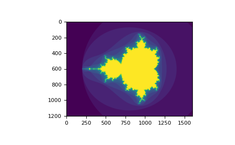
You can look at the following example to see how to use Boolean index generation Mandelbrot set Image of:
>>> import numpy as np
>>> import matplotlib.pyplot as plt
>>> def mandelbrot(h, w, maxit=20, r=2):
...     """Returns an image of the Mandelbrot fractal of size (h,w)."""
...     x = np.linspace(-2.5, 1.5, 4*h+1)
...     y = np.linspace(-1.5, 1.5, 3*w+1)
...     A, B = np.meshgrid(x, y)
...     C = A + B*1j
...     z = np.zeros_like(C)
...     divtime = maxit + np.zeros(z.shape, dtype=int)
...
...     for i in range(maxit):
...         z = z**2 + C
...         diverge = abs(z) > r                    # who is diverging
...         div_now = diverge & (divtime == maxit)  # who is diverging now
...         divtime[div_now] = i                    # note when
...         z[diverge] = r                          # avoid diverging too much
...
...     return divtime
>>> plt.imshow(mandelbrot(400, 400))
The second way to index using Boolean values is more similar to integer indexes; For each dimension of the array, we give a one-dimensional Boolean array and select the slice we want:
>>> a = np.arange(12).reshape(3, 4)
>>> b1 = np.array([False, True, True])         # first dim selection
>>> b2 = np.array([True, False, True, False])  # second dim selection
>>>
>>> a[b1, :]                                   # selecting rows
array([[ 4,  5,  6,  7],
       [ 8,  9, 10, 11]])
>>>
>>> a[b1]                                      # same thing
array([[ 4,  5,  6,  7],
       [ 8,  9, 10, 11]])
>>>
>>> a[:, b2]                                   # selecting columns
array([[ 0,  2],
       [ 4,  6],
       [ 8, 10]])
>>>
>>> a[b1, b2]                                  # a weird thing to do
array([ 4, 10])
Note that the length of the one-dimensional Boolean array must be consistent with the length of the dimension (or axis) to be sliced. In the previous example, b1 has a length of 3 (a in the number of rows), and b2 (length 4) is suitable for the second axis (column) a of the index.
ix_ () function
Should ix_ The function can be used to combine different vectors to obtain the results of each n-uplink. For example, if you want to calculate all a+b*c of all triples extracted from each of vectors a, B, and c:
>>> a = np.array([2, 3, 4, 5])
>>> b = np.array([8, 5, 4])
>>> c = np.array([5, 4, 6, 8, 3])
>>> ax, bx, cx = np.ix_(a, b, c)
>>> ax
array([[[2]],

       [[3]],

       [[4]],

       [[5]]])
>>> bx
array([[[8],
        [5],
        [4]]])
>>> cx
array([[[5, 4, 6, 8, 3]]])
>>> ax.shape, bx.shape, cx.shape
((4, 1, 1), (1, 3, 1), (1, 1, 5))
>>> result = ax + bx * cx
>>> result
array([[[42, 34, 50, 66, 26],
        [27, 22, 32, 42, 17],
        [22, 18, 26, 34, 14]],

       [[43, 35, 51, 67, 27],
        [28, 23, 33, 43, 18],
        [23, 19, 27, 35, 15]],

       [[44, 36, 52, 68, 28],
        [29, 24, 34, 44, 19],
        [24, 20, 28, 36, 16]],

       [[45, 37, 53, 69, 29],
        [30, 25, 35, 45, 20],
        [25, 21, 29, 37, 17]]])
>>> result[3, 2, 4]
17
>>> a[3] + b[2] * c[4]
17
You can also implement reduce as follows:
>>> def ufunc_reduce(ufct, *vectors):
...    vs = np.ix_(*vectors)
...    r = ufct.identity
...    for v in vs:
...        r = ufct(r, v)
...    return r
Then use it as:
>>> ufunc_reduce(np.add, a, b, c)
array([[[15, 14, 16, 18, 13],
        [12, 11, 13, 15, 10],
        [11, 10, 12, 14,  9]],

       [[16, 15, 17, 19, 14],
        [13, 12, 14, 16, 11],
        [12, 11, 13, 15, 10]],

       [[17, 16, 18, 20, 15],
        [14, 13, 15, 17, 12],
        [13, 12, 14, 16, 11]],

       [[18, 17, 19, 21, 16],
        [15, 14, 16, 18, 13],
        [14, 13, 15, 17, 12]]])
With ordinary UFUNC Compared with reduce, the advantage of this version of reduce is that it uses Broadcasting rules To avoid creating an array of parameters whose output size is multiplied by the number of vectors.
Index with string
see also Structured array.
Tips and tricks
Here, we provide a short and useful list of tips.
Auto shaping
To change the dimension of the array, you can omit one of the sizes that will be automatically derived later:
>>> a = np.arange(30)
>>> b = a.reshape((2, -1, 3))  # -1 means "whatever is needed"
>>> b.shape
(2, 5, 3)
>>> b
array([[[ 0,  1,  2],
        [ 3,  4,  5],
        [ 6,  7,  8],
        [ 9, 10, 11],
        [12, 13, 14]],

       [[15, 16, 17],
        [18, 19, 20],
        [21, 22, 23],
        [24, 25, 26],
        [27, 28, 29]]])
Vector stack
How do we construct a two-dimensional array from a list of equally sized row vectors? In MATLAB, this is easy: if x and y are two vectors of the same length, you just need to do m=[x;y]. Here, the working principle of NumPy's pass function column_stack, dstack, hstack and vstack, visual dimension must be done in stacking. For example:
>>> x = np.arange(0, 10, 2)
>>> y = np.arange(5)
>>> m = np.vstack([x, y])
>>> m
array([[0, 2, 4, 6, 8],
       [0, 1, 2, 3, 4]])
>>> xy = np.hstack([x, y])
>>> xy
array([0, 2, 4, 6, 8, 0, 1, 2, 3, 4])
The logic behind these functions with more than two dimensions can be strange.
You can also have a look
histogram
Histogram the NumPy function applied to the array returns a pair of vectors: the histogram of the array and the vector of the bin edge. Note: matplotlib also has a function to build histograms different from those in NumPy (called in Matlab). The main difference is that pyrab.hist automatically draws histograms, while numpy.histogram only generates data.
>>> import numpy as np
>>> rg = np.random.default_rng(1)
>>> import matplotlib.pyplot as plt
>>> # Build a vector of 10000 normal deviates with variance 0.5^2 and mean 2
>>> mu, sigma = 2, 0.5
>>> v = rg.normal(mu, sigma, 10000)
>>> # Plot a normalized histogram with 50 bins
>>> plt.hist(v, bins=50, density=True)       # matplotlib version (plot)
>>> # Compute the histogram with numpy and then plot it
>>> (n, bins) = np.histogram(v, bins=50, density=True)  # NumPy version (no plot)
>>> plt.plot(.5 * (bins[1:] + bins[:-1]), n)
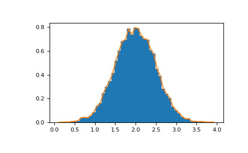
Using Matplotlib > = 3.4, you can also use plt.stairs(n, bins)