12. Image smoothing
12.1 objectives
- Learn: - blur images with various low-pass filters - apply custom filters to images (2D convolution)
12.2 # 2D convolution (image filtering)
Like the one-dimensional signal, various low-pass filters (LPF) and high pass filters (HPF) can also be used to filter the image. LPF helps to eliminate noise and blur the image. The HPF filter helps to find edges in the image.
OpenCV provides a function cv Filter 2D to convolute the kernel with the image. For example, we will try to average filter the image. The 5x5 average filter core is as follows:
The following is cv Filter2d function prototype and specific parameters:
dst=cv.filter2D(src, ddepth, kernel[, dst[, anchor[, delta[, borderType]]]])
| parameter | describe |
| src | The original image, that is, the input image matrix |
| ddepth | The required depth of the target image is consistent with the input image by default |
| kernel | Convolution kernel (or equivalent to correlation kernel), convolution kernel function and single channel floating-point matrix need to be declared in advance; If you want to apply different kernels to different channels, use split to split the image into separate color planes, and then process them separately. |
| dst | The target image has the same size and number of passes as the original image |
| anchor | The anchor point of the convolution kernel indicates the relative position of the filter point in the kernel; The anchor shall be located in the core; The default value is (- 1, - 1), which means that the anchor is located in the center of the kernel. |
| detal | Add optional values to the filtered pixels before storing them in the dst. Similar to offset. |
| borderType | The method of how to fill pixels by convolution to the image boundary is the pixel extrapolation method. See BorderTypes |
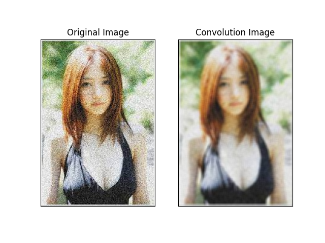
The operation is as follows: keep the kernel on one pixel, add all 25 pixels lower than the kernel, take the average value, and then replace the central pixel with the new average value. It will continue this operation for all pixels in the image. Try this code and check the result:
import cv2 as cv
import matplotlib.pyplot as plt
import numpy as np

img = plt.imread('001.jpg')
kernel = np.ones((5, 5), np.float32) / 25  # Kernel function normalization
dst = cv.filter2D(img, -1, kernel)
plt.subplot(121), plt.imshow(img, 'gray'), plt.title('Original Image')
plt.xticks([]), plt.yticks([])
plt.subplot(122), plt.imshow(dst, 'gray'), plt.title('Convolution Image')
plt.xticks([]), plt.yticks([])
plt.show()
The operation results are as follows:
12.3 image blur (image smoothing)
Image blur is realized by convoluting the image with the low-pass filter core. This is useful for eliminating noise. It actually eliminates high-frequency parts (e.g. noise, edges) from the image. Therefore, the edges are somewhat blurred in this operation. (some blur techniques can also not blur the edge). OpenCV mainly provides four types of fuzzy technology.
12.3.1 average
This is accomplished by convoluting the image with the normalized frame filter. It only gets the average value of all pixels under the kernel area and replaces the central element. This is through the function cv Blur () or CV Boxfilter() completed. Check the documentation for more details about the kernel. We should specify the width and height of the kernel. 3x3 normalized frame filter is as follows:
Note: if you do not want to use standardized frame filters, please use cv boxFilter(). Pass the parameter normalize =False to the function.
The following is cv Description and parameter setting of blur() function:
cv.blur(src, ksize, dst=None, anchor=None, borderType=None):
| parameter | describe |
| src | The original image, that is, the input image matrix |
| ksize | The convolution kernel size does not require filter2D to set all parameters of the kernel, but only the convolution kernel size; |
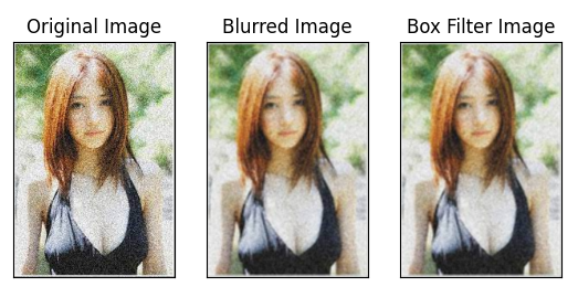
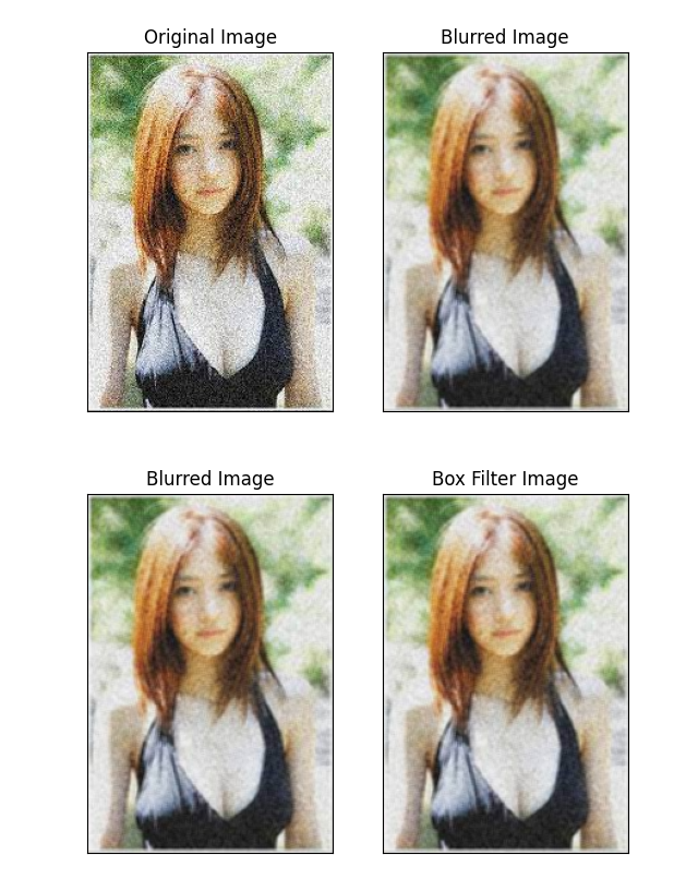
Take a look at the following example demonstration, whose kernel size is 3x3:
import cv2 as cv
from matplotlib import pyplot as plt

img = plt.imread('001.jpg')
blur = cv.blur(img, (3, 3))  # Mean filtering
box_filter = cv.boxFilter(img, 0, (3, 3))

plt.subplot(131), plt.imshow(img), plt.title('Original Image')
plt.xticks([]), plt.yticks([])

plt.subplot(132), plt.imshow(blur), plt.title('Blurred Image')
plt.xticks([]), plt.yticks([])

plt.subplot(133), plt.imshow(box_filter), plt.title('Box Filter Image')
plt.xticks([]), plt.yticks([])

plt.show()
The operation results are as follows:
12.3.2 Gaussian filtering
In this case, instead of the box filter, Gaussian kernel is used. This is through the function cv Completed by Gaussian blur(). We should specify the width and height of the kernel, which should be positive and odd. We should also specify the standard deviations in the X and Y directions, sigma X and sigma y, respectively. If only sigma x is specified, then sigma y will be the same as sigma X. If both are zero, the calculation is based on the kernel size. Gaussian blur is very effective for removing Gaussian noise from images.
If necessary, you can use the function cv Getgaussian kernel() creates a Gaussian kernel.
The following is the Gaussian filter function and Parameter Description:
cv.GaussianBlur(src, ksize, sigmaX, dst=None, sigmaY=None, borderType=None):
| parameter | describe |
| src | input image |
| ksize | Gaussian kernel size |
| sigmaX | Gaussian kernel standard derived variance |
| sigmaY | The default setting is 0, which will be consistent with sigmaX; If both semax and semay are 0, ksize will be calculated Width and ksize Height to output the size of sigma X and sigma y; |
| borderType | Filling method of convolution at image edge |
You can modify the above code to achieve Gaussian blur:
import cv2 as cv
from matplotlib import pyplot as plt

img = plt.imread('001.jpg')
kernel = (3, 3)
blur = cv.blur(img, kernel)  # Mean filtering
box_filter = cv.boxFilter(img, 0, kernel)
gauss_blur = cv.GaussianBlur(img, kernel, 0)

images = [img, blur, box_filter, gauss_blur]
titles = ['Original Image', 'Blurred Image', 'Box Filter Image',
          'Gaussian Blurred Image']

for i in range(2):
    plt.subplot(2, 2, 2 * i + 1)
    plt.imshow(images[i], 'gray')
    plt.title(titles[i])
    plt.xticks([]), plt.yticks([])

    plt.subplot(2, 2, 2 * i + 2)
    plt.imshow(images[i + 1], 'gray')
    plt.title(titles[i + 1])
    plt.xticks([]), plt.yticks([])

plt.show()
The operation results are as follows:
12.3.3 # median filtering
Here, the function cv Medianblur() extracts the median value of all pixels under the kernel area and replaces the central element with the median value. This is very effective for eliminating salt and pepper noise in the image. Interestingly, in the above filter, the central element is a newly calculated value, which can be a pixel value or a new value in the image. However, in median blur, the central element is always replaced by some pixel values in the image. Effectively reduce noise. Its kernel size should be a positive odd integer.
The following is cv Medianblur() function prototype and specific parameters:
median = cv.medianBlur(src, ksize, dst=None):
| parameter | describe |
| src | input image |
| ksize | Filter core size |
| dst | The output image has the same size and number of passes as the original image |
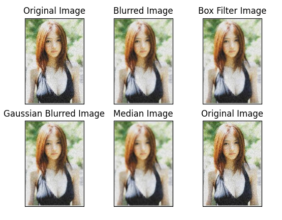
In this demonstration, I added 50% noise to the original image and applied median blur. Inspection results:
import cv2 as cv
from matplotlib import pyplot as plt

img = plt.imread('001.jpg')
kernel = (3, 3)
blur = cv.blur(img, kernel)  # Mean filtering
box_filter = cv.boxFilter(img, 0, kernel)
gauss_blur = cv.GaussianBlur(img, kernel, 0)
median = cv.medianBlur(img, 5)

images = [img, blur, box_filter, gauss_blur, median, img]
titles = ['Original Image', 'Blurred Image', 'Box Filter Image',
          'Gaussian Blurred Image', 'Median Image', 'Original Image']

for i in range(2):
    plt.subplot(2, 3, i * 3 + 1)
    plt.imshow(images[i * 3], 'gray')
    plt.title(titles[i * 3])
    plt.xticks([]), plt.yticks([])

    plt.subplot(2, 3, i * 3 + 2)
    plt.imshow(images[i * 3 + 1], 'gray')
    plt.title(titles[i * 3 + 1])
    plt.xticks([]), plt.yticks([])

    plt.subplot(2, 3, i * 3 + 3)
    plt.imshow(images[i * 3 + 2], 'gray')
    plt.title(titles[i * 3 + 2])
    plt.xticks([]), plt.yticks([])

plt.show()
The operation results are as follows:
12.3.4 bilateral filtering
cv.bilateralFilter() is very effective in removing noise while keeping the edges clear and sharp. However, this operation is slower than other filters. We have seen that the Gaussian filter takes the neighborhood around the pixel and finds its Gaussian weighted average. Gaussian filter is only a function of space, that is, nearby pixels will be considered when filtering. It does not consider whether pixels have almost the same intensity. It does not consider whether the pixel is an edge pixel. So it also blurs the edges, which we don't want to do.
The bilateral filter also adopts Gaussian filter in space, but there is another Gaussian filter, which is a function of pixel difference. The Gaussian function of space ensures that only the blur of nearby pixels is considered, while the Gaussian function of intensity difference ensures that only those pixels whose intensity is similar to that of the central pixel are considered. Because the pixel intensity of the edge changes greatly, the edge can be retained.
The following example shows the use of bilateral filters (for more information on parameters, visit docs).
cv.bilateralFilter(src, d, sigmaColor, sigmaSpace, dst=None, borderType=None)
Of which:
| parameter | describe |
| src | input image |
| d | If the neighborhood diameter of the filter kernel function is negative, it is calculated according to sigmaSpace; |
| sigmaColor | sigma parameter (range) of filtered color space |
| sigmaSpace | sigma parameters of coordinate space (airspace) |
| dst | Output image |
| borderType | Image convolution boundary filling method |
12.4 other resources
Details about bilateral filtering are here
Welcome to leave a message in the comment area to explore the mystery of OpenCV's path to God.
By the way, give me an attention, a praise and a collection. Let's go to the altar together.