1. opecv reading and displaying images

Reading and displaying images is the simplest and most basic operation in opencv. Although it can be implemented using only two simple API s, there are some small details that should be paid attention to`

#include<opencv2/opencv.hpp>
using namespace std;
using namespace cv;

int main()
{
	Mat src = imread("C:/Users/51731/Desktop/2.jpeg");
	if (!src.data)
	{
		cout << "no image" << endl;
		return 0;
	}

	namedWindow("frame_1", WINDOW_AUTOSIZE);
	imshow("frame_1", src);
	waitKey(0);
	return 1;
}

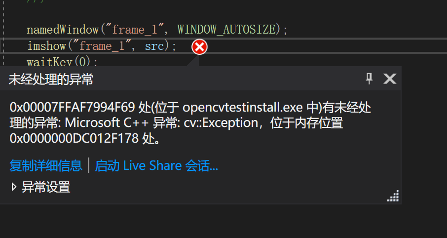
Use the cv::imread() method to read out a photo. The type returned by this function is a Mat type. The characteristics and usage of this data type will be recorded in the next section. When using opencv in C + + to read images, it is best to use if to judge whether the photos are read successfully after reading. Because if there is an error in image reading, the error message of C + + is as shown in the figure below. If the program structure is simple and clear, this Bug is easy to find and solve, but if the program structure is complex, it will be difficult to find such errors.

Besides, namedWindow opens a new window. The size of the window can be adjusted using the second parameter. Use the created window on the first parameter of imshow function to display the image on the created window. If the window is not created in advance, imshow will generate a new window with the string entered in the first parameter as the window name. waitKey() allows the window to be continuously displayed on the window. You can use parameters to adjust the dwell time of the current window. If it is

• waitkey(0): press any key to continue.
• waitkey(500): wait 500 milliseconds before continuing.

Reading and displaying images is roughly like this, which is easy to understand and master.

2. Nature and use of mat object

Mat object is a very important data type provided by Opencv. It provides us with a useful container to carry the images read from the hard disk. Its main purpose is to store array s of any size.

The cv::Mat class is used to represent dense arrays of any number of dimensions. In
this context, dense means that for every entry in the array, there is a data value stored
in memory corresponding to that entry, even if that entry is zero

It can be found from the above references that the data type Mat is used to store deny arrays. If we encounter a large sparse matrix and use the Mat data type for storage, it is certainly feasible in theory, but it will cause a lot of memory consumption than necessary. Most of the sparse matrices are 0. For this problem, Opencv also provides another data type cv::SparseMat() to deal with sparse matrices.
Common properties of cv::Mat object:

• Rows: indicating the number of rows in the matrix
• Columns: indicating the number of columns in the matrix
• dims: indicating the dimension of the matrix
• flag: flags element signaling the contents of the array
  What needs to be recorded is that flag is an int variable, and each digit represents a unique meaning. For details, please refer to This article
• PTR < > (i, j): get the pointer of row i and column j. < > Pointer type in.
  Mat also has many attributes, but these attributes are more commonly used. In the following notes, we will also use these attributes of mat a lot.

2.1 creating Mat objects

There are many ways to create a Mat object. The first is to directly create a Mat type variable and assign it a value.

Mat src = (Mat_<int>(3,3) << -1, 0, -1, 0, 5, 0, -1, 0, -1);

Just like the above code, it creates a Mat with a size of 3 * 3 and a member type of Int. This method can be used to create a small Mat object with a fixed value. It is more suitable for creating small convolution kernels.

In addition to this method, you can also use

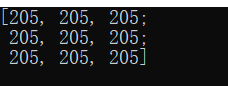
Mat src;
src.create(3,3,CV_8U);

The above code creates a 3 * 3, and the data type is cv_ Mat object of 8U src. However, the value in the current src variable of mat type is random according to the data type. Like cv_ The result of 8U is:

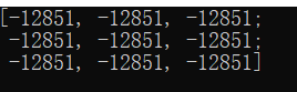
But if it's a CV_16S, the value of the generated Mat object becomes:

(these small details may not seem very useful now, but they may become the key to debug at some point in the future.)
When setting the size of Mat, in addition to the above code, you can also use Size(3,3) to get the same effect as the above code.

new_.create(Size(3, 3), CV_16S);

The values in the Mat object created by the Create method are "meaningless". If you want to create a matrix with all 1 or all 0, you can do the following:

src = Mat::ones(Size(3, 3), CV_16S);
src = Mat::zeros(Size(3, 3), CV_16S);

It is often encountered in actual operation that a Mat object with the same size as an image needs to be created. At this time, you can first obtain the rows and cols of the image, and then use the Create method to create it

Mat src = imread("C:/Users/Desktop/2.jpeg");
	if (!src.data)
	{
		cout << "no image" << endl;
		return 0;
	}
	int src_rows = src.rows;
	int src_cols = src.cols;
	Mat new_mat;
	new_mat.create(src_rows, src_cols, CV_16S);
	cout << "number of rows:" << new_mat.rows << endl;
	cout << "number of cols:" << new_mat.cols << endl;

Of course, there are other ways not to use create:

Mat new_mat(src.size(), src.type());

In the above way, you can define the size and type of a new Mat object when defining it.

2.2 deep and shallow copy of mat object

In addition to the above common cases, we can also copy an existing Mat object as a new one
Object. However, when copying, you should pay attention to the difference between deep and shallow copies. Deep and shallow copies will not be repeated here. There are several common methods to copy Mat objects in Opencv. Although the final results are consistent, there are some minor details that can be noted, which may play a role in improving computing efficiency and efficient resource allocation.

• =: assignment by assignment number is a typical shallow copy. Changing the Mat from any shallow copy will change all its related mats
• src.clone(): this function provides a deep copy method, which will directly apply for a new memory address in memory.
• src. Copy to (dst): the parameter dst is the copy result. This function is also a deep copy method, but different from clone, whether to apply for new memory space depends on whether the sizes of dst and Src are consistent. If the size is consistent, it will not be applied. If it is inconsistent, it will open up a new space.

2.3 pointer operation of Mat object (operation of elements in Mat)

Using pointers to manipulate and process elements in Mat is often used in image processing algorithms. A large number of image algorithms process images from pixels. Opencv can use: pointer = src PTR < uchar > (), if you want to read the first line of src, you can use pointer = src ptr<uchar>(0). Similarly, if you want the elements in the matrix to operate, you can also use a similar method. For example, now you want to operate the data in row 0 and column 0 with the data in the first column of row 0. We can:

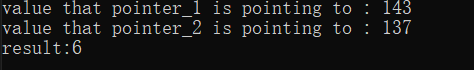
//First obtain the pointers of the two elements of row 0, column 0 and row 0, column 1, and then calculate

	const uchar* pointer_1 = src.ptr<uchar>(0, 0); // pointer_1
	const uchar* pointer_2 = src.ptr<uchar>(0, 1); // pointer_2


	printf("value that pointer_1 is pointing to : %d\n", *pointer_1);
	printf("value that pointer_2 is pointing to : %d\n", *pointer_2);

	uchar var_1 = *pointer_1 - *pointer_2;

	printf("result:%d\n", var_1);

The results obtained are as follows:

In fact, I don't quite understand why the type of pointer must be uchar. Because I tried int, double, uint and other data types, the results seem to be random numbers.

3. Improve image contrast

After the above operations on Mat objects and the basic methods of reading and writing photos, you can use these knowledge points to improve the image contrast. The principle of image contrast enhancement is to use a fixed convolution kernel to convolute with the original image, so that the edge and contour of the image are more obvious.
Because it involves the operation between pixels, the pointer to obtain each pixel mentioned above will be used.

#include<opencv2/opencv.hpp>

using namespace std;
using namespace cv;


int main()
{

	Mat src = imread("1.jpeg");
	if (!src.data)
	{
		printf("no image");
		return -1;
	}

	//Cycle through each pixel in the image
	int nchannel = src.channels();
	int img_rows = src.rows;
	int img_cols = src.cols * src.channels();
	cout << "img_row" << img_rows << endl;
	cout << "img_cols" << img_cols << endl;
	Mat result_img = Mat::zeros(src.size(), src.type()); // Create a new Mat to store the processed photos.

	//Suppose there is a convolution kernel of 3 * 3, and the weight in the kernel has been fixed
	for (int row = 1; row < img_rows - 1; row++) //Traverse each line
	{

		const uchar* previous = src.ptr<uchar>(row - 1); //Find the pointer position of the current line, the previous line and the next line.
		const uchar* current = src.ptr<uchar>(row); // Pointer position of the current row.
		const uchar* next = src.ptr<uchar>(row + 1); //Pointer position of the next line.
		uchar* output_pointer = result_img.ptr<uchar>(row);


		for (int col = nchannel; col < img_cols; col++)
		{
#			//The value of the current pixel after convolution.
			output_pointer[col] = saturate_cast<uchar>(5 * current[col] - (current[col - nchannel] + current[col + nchannel] + previous[col] + next[col]));

		}
	}

	namedWindow("original", CV_WINDOW_AUTOSIZE);
	imshow("original", src);

	namedWindow("test_frame_1", CV_WINDOW_AUTOSIZE);
	imshow("test_frame_1", result_img);
	waitKey(0);
	return 0;
}

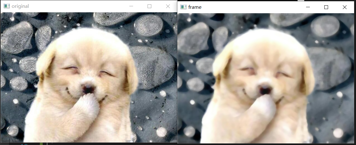
Through the above code, you can get an effect as shown in the figure below

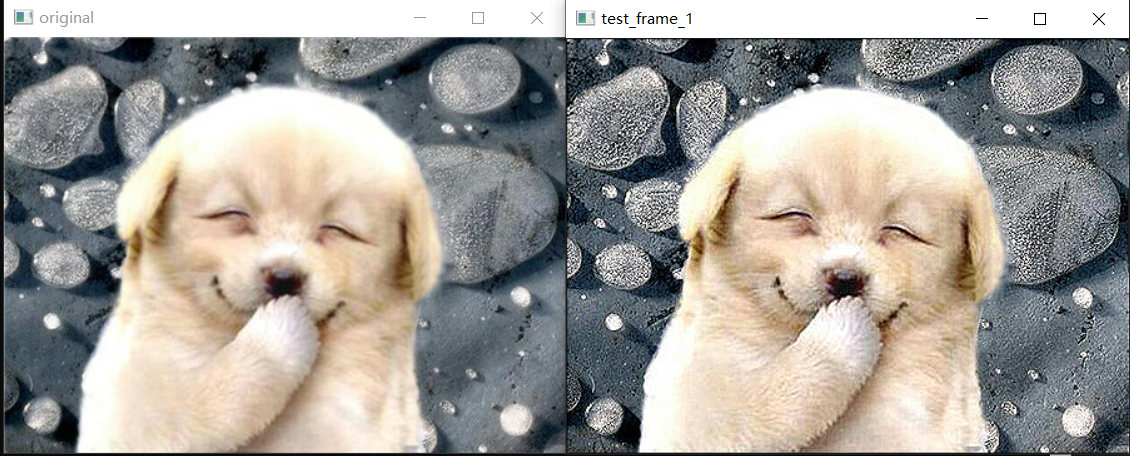
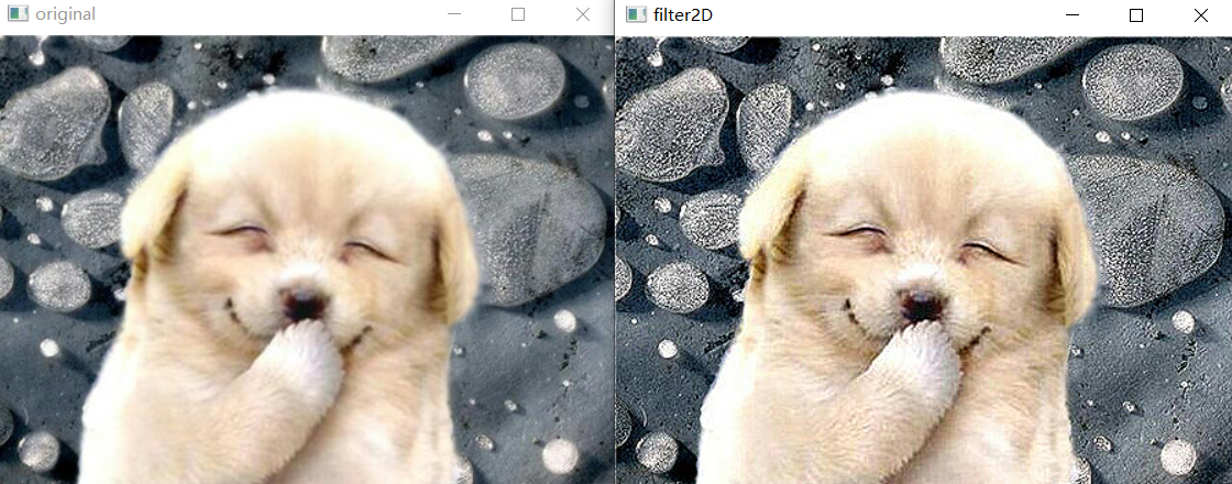
It is obvious that after the contrast is improved, the details of the image will be much more obvious than the previous image. But you will find that the above code may be too lengthy. Opencv provides a simple way to complete the filtering operation: filter2D(). The effect of this method is almost no big gap with the above code.

	Mat dst; 
	Mat kernel = (Mat_<int>(3, 3) << 0, -1, 0, -1, 5, -1,0,-1,0);
	filter2D(src, dst,-1, kernel);

4. Image blending

The image mixing operation is to fuse two photos into one photo according to different intensities. It is widely used in image processing. For example, add weighted method can be used to draw the mask output by mask rcnn onto the original image. The essence of this method is to add the corresponding elements of each of the two array s according to a certain weight.

cv::addWeighted() Perform element-wise weighted addition of two arrays (alpha blending)

The theoretical support behind this method is:

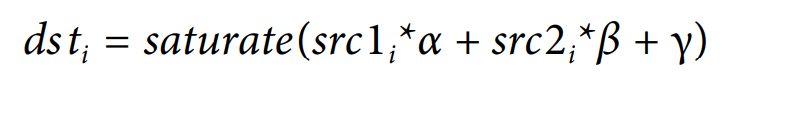
Where src1 is the first input image and src2 is the second input image, α and β Corresponding to the intensity of the addition of the two images, γ Offset added to weighted sum. Next, we will do several experiments and record the impact of changing parameters on the final results.

In fact, it is easy to find out according to the formula α and β The impact of change on the results is nothing more than when α The larger s RC1 is more obvious in the results, and the larger s RC2 in Beta is more obvious. But what is the effect of changing gamma. In order to observe the change caused by the change of a variable, a trackbar can be used to observe the impact of the change. The specific code can be shown in the figure below:

#include<opencv2/opencv.hpp>

using namespace std;
using namespace cv;


void weighted(int, void*);

Mat src = imread("1.jpeg");
Mat src_1 = imread("2.jpeg");
double alpha = 0.5;
double beta = 0.5;
int gamma_ = 2;
Mat dst;


int main()
{
	if (!(src.data && src_1.data ))
	{
		printf("no image");
		return -1;
	}
	namedWindow("original"); //Display original figure 1
	namedWindow("original_1"); //Display original figure 2
	namedWindow("weighted"); // Show weighted graph

	imshow("original", src);
	imshow("original_1", src_1);
	resize(src_1, src_1, src.size(), 0.5, 0.5);
	cout << "size of src_1" << src_1.size() << endl;
	cout << "size of src" << src.size() << endl;
	//Use this function to call the weighted function to realize the function of dragging bar to adjust parameters.
	createTrackbar("gamma", "weighted", &gamma_, 20, weighted); 

	waitKey(0);
	return 1;
	
}

void weighted(int, void*)
{
	addWeighted(src, alpha, src_1, beta, gamma_, dst);
	imshow("weighted", dst);
}

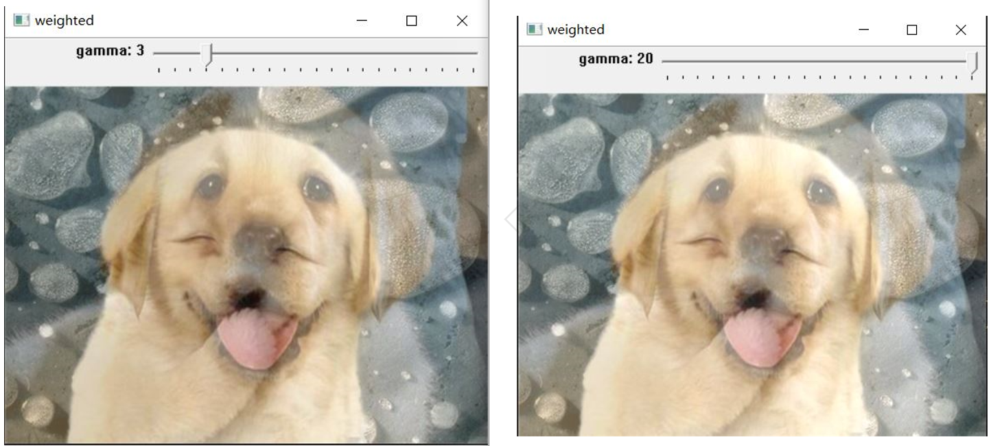
It should be noted that using the addweighted function, the size of the two images should be the same, otherwise an error will occur. Therefore, before adding, resize the two photos with unequal sizes. Then the results are shown in the figure below:
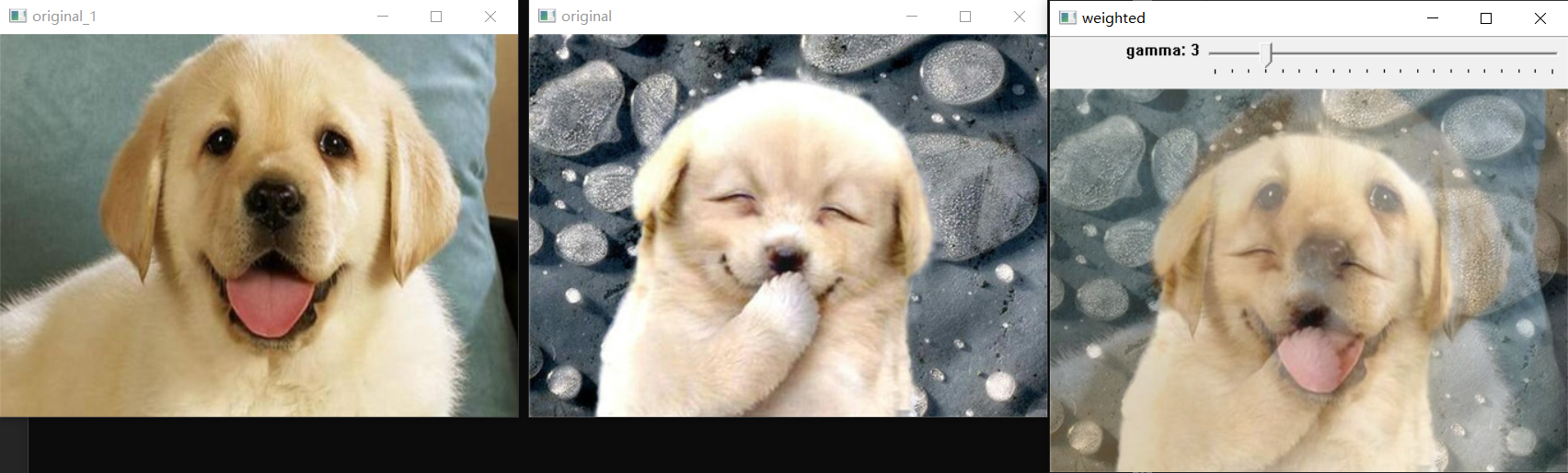The following figure shows the difference when the intensity of the offset gamma is 3 and 20. It can be seen that when the gamma value is relatively large, the brightness of the image will be greater than when the gamma is small. That is, the gamma value is added to each pixel value.

5. Draw basic geometric image

The API for drawing basic images is relatively boring, but these basic APIs play a very important role in the subsequent image processing. For example, in object detection, we usually need to frame the objects in the original image. At this time, we will use the drawing tools of these images, which is also the basic operation of image processing.

5.1 points

Point usually uses Point(a,b) to define a point. The reason why it is recorded separately is that there are many drawing tools that need to provide the positions of multiple points to draw the desired graph. So it can be said to be a very basic but important API. The specific application methods are as follows:

	Point a = Point(1, 2);
	cout << a << endl;

The result of the above code should be:

Through the above code, we can find that point can be understood as a data type provided by OpenCV, just like Mat.

5.2 wiring

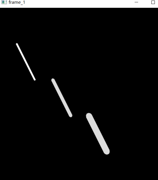
The API and usage of line drawing are as follows:

int main()
{

	Mat mat = Mat::zeros(300, 300, CV_8U);
	Point point_a = Point(100, 100);
	Point point_b = Point(200, 200);
	Scalar color = Scalar(255,255,255);
	line(mat,point_a,point_b,Scalar(255,255,255),LINE_8);
	namedWindow("frame_1");
	imshow("frame_1", mat);
	waitKey(0);
	return 1;

}

API:

line(mat,point_a,point_b,color,LINE_8);
mat: It's the target image. To put it simply, draw on that picture.
point_a / point_b: Two points needed to draw a line.
color : The color of the line is a Scalar Variable of type.
LINE_8 Is a type of line. stay opencv Three types of wires are provided in

 - LINE_8
 - LINE_4
 The difference between the above two is in thickness, which is obvious LINE_8 Than LINE_4 crude
 - LINE_AA: Anti-Aliasing 

The following figure shows the effects of three line types, line from top to bottom_ 4, LINE_ 8, LINE-AA.

5.3 rectangle

The method of drawing a rectangle is very similar to that of drawing a straight line. To draw a straight line, you need to use Point to define two points, and to draw a rectangle, you need to define a rectangle first.
Define rectangle API:

Rect rect = Rect(200, 100, 150, 100);
The first two parameters represent the coordinates of the upper left point of the rectangle, and the last two points represent the coordinates of the lower right points.

Then, the API for drawing rectangles can be basically the same as drawing straight lines, so I won't go into too much detail.

	Rect rect = Rect(200, 100, 150, 100);
	Scalar color = Scalar(255, 0, 0);
	rectangle(src, rect, color, LINE_8);

5.4 ellipse

The API for drawing ellipses is slightly more complex than the first two. This API can not only be used to draw ellipses, but also draw arcs or circles according to given parameters. The API of ellipse is roughly as follows:

void ellipse(InputOutputArray img, Point center, Size axes,
                        double angle, double startAngle, double endAngle,
                        const Scalar& color, int thickness = 1,
                        int lineType = LINE_8, int shift = 0);
Meaning of parameters:
src: On which map do you need to draw.
center : center of a circle.
Size axes: Major axis and minor axis.
angle:Tilt angle.
startAngle: Start angle
endAngle: End angle.
color : Color.
thickness: The line is thick.

Where the unit of angle parameter is degrees (°), not radians. It represents the inclination angle of the long axis of the ellipse. Specifically, it represents the angle that the long axis deviates from the horizontal direction (X axis) counterclockwise.

The angle is the angle (in degrees) of the major axis, which is measured
counterclockwise from horizontal (i.e., from the x-axis).

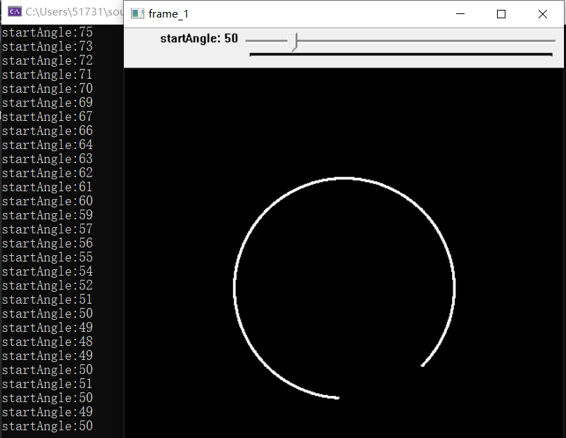
Changing the angle parameter can adjust the tilt angle of the ellipse in the figure. Adjusting startAngle and endAngle can adjust the size of the arc. When startAngle = 0 and endAngle = 360, it is an ellipse. Through the actual code demonstration, you can more clearly see the impact of different startAngle and endAngle on the results.

Similarly, the startAngle and endAngle indicate (also in degrees) the angle for the arc to start and for it to fin‐
ish. Thus, for a complete ellipse, you must set these values to 0 and 360, respectively.

#include<opencv2/opencv.hpp>

using namespace std;
using namespace cv;

 
void modification(int, void*);
int startAngle = 270;
int endAngle = 360;
Mat src = Mat::zeros(500, 500, CV_8U);
int main()
{

	namedWindow("frame_1");
	createTrackbar("startAngle","frame_1",&startAngle,endAngle,modification);
	modification(0,0);
	waitKey(0);
	return 1;
}

void modification(int, void*)
{	
	cout << startAngle << endl;
	ellipse(src, Point(250, 250), Size(src.rows / 4, src .cols / 4), 45, startAngle, endAngle, Scalar(255, 255, 255), 2, LINE_8);
	imshow("frame_1", src);
}

Adjust startAngle through trackbar to observe the difference between different startAngle and EndAngle. The following figure shows the image when startAngle = 180 and endAngle = 360:
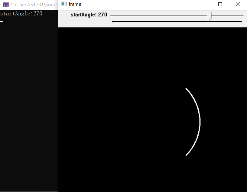It can be observed that the image at this time is only an arc. By adjusting startAngle to a smaller value, the shape of the ellipse (the parameter set here will output a circle) becomes more and more complete.

The following figure can intuitively explain the meaning of each parameter in this API.

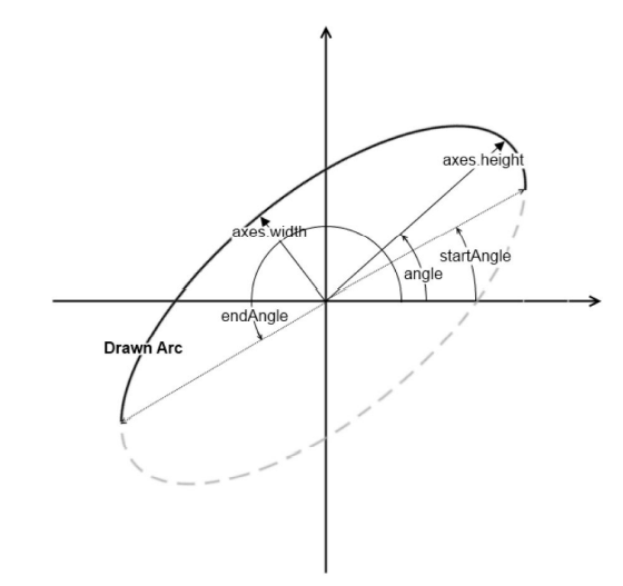
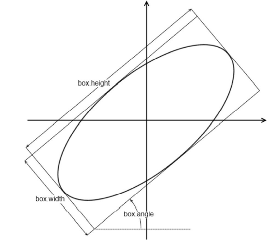
In addition to the above operations, we can use a rectangle to fit the ellipse, as shown in the following figure:

6. Linear filtering and nonlinear filtering

Filtering operation is widely used in image processing. The function of filtering is to do some mild image blur, make the details more prominent, find out the boundary, remove noise and so on. Generally, the filtering operation can be used before and after image processing,

filter images in order to add soft blur, sharpen details, accentuate edges, or remove noise.

Some basic filtering methods are briefly recorded below.

6.1 linear filtering

The most common one is linear filtering, which can be understood as the weighted sum of adjacent pixel values. The weighted weight is determined by another smaller matrix, usually called kernel or filter. The principle is very similar to the forward propagation principle of kernel convolutional neural network. The following figure is the expression of linear filtering:

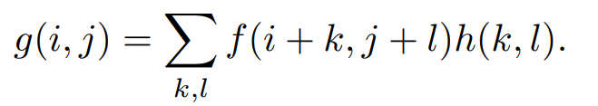
According to the desired effect, appropriately changing the value and size of the core will have a very different effect. As demonstrated above, improving image contrast is a practical application of linear filtering. Linear filtering can be implemented using filter2D, because it has been mentioned earlier, so it will not be repeated here. The value of kernel is usually cardinality. In the actual development process, because linear filtering is used, each pixel needs K * K operations, and K is the size of the kernel. Therefore, it can be seen that although conventional linear filtering is feasible, its efficiency is low. Therefore, separable kernel is sometimes used to replace the traditional convolution kernel. Separable convolution kernel means that the convolution is performed by using a convolution direction to check the horizontal direction, and then using a convolution check image in the vertical direction to convolute, so that the calculation amount of each pixel is reduced from K^2 to 2* K.

6.2 nonlinear filtering

6.2.1 median filtering

Median filtering is to select the median of adjacent pixels to replace the value of the current pixel. The principle of median filter is relatively simple, so it has become a major advantage. Median filter can be completed in linear time. API of median filter:

medianBlur(src,dst,ksize);
Parameters:
src: Original.
dst : Matrix for storing results.
ksize : kernel The size of the.

The median filtering effect of 7 * 7 is as follows:

However, its disadvantage is also very obvious, that is, using a value instead of each output pixel has no particularly ideal effect on Gaussian noise. Therefore, weighted median filter can be used to make up for this problem. The principle of weighted median filter is relatively simple: the use times of the pixel are determined according to the distance between the pixel and the central pixel.

Another possibility is to compute a weighted median, in which each pixel is used a number of times depending on its distance from the center.

6.2.2 bilateral filtering

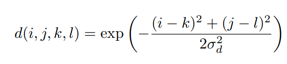
In fact, bilateral filtering has many similarities with the filtering algorithm mentioned above. Its main principle is to use the weighted average method: the weighted average value of pixels around pixel a is used to represent the value of pixel a. However, the biggest difference between bilateral filtering and other filtering algorithms is that its weight takes into account not only the distance between the pixel and the central pixel, but also some differences of the pixel itself. Formally, the output of bilateral filtering shall be as follows:

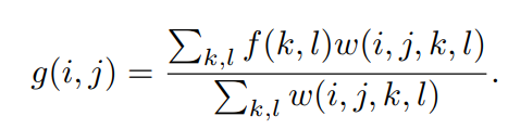
The weight w is composed of two cores, one is the domain kernel and the other is the range kernel. Where the expression of domain kernel is

range kernel is expressed as:

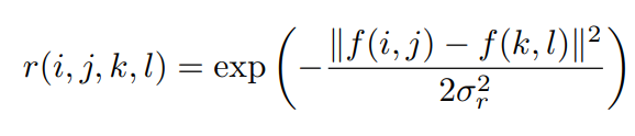
Where f(i,j) and f (k,l) represent the intensity of pixels (i,j) and pixels (k,l). The weight of bilateral filter is the product of the above two:

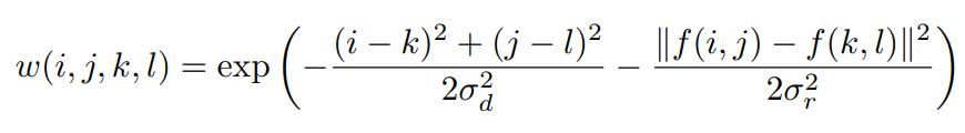
Therefore, the advantage of bilateral filter is that when the change value of pixel is very small (the change of pixel intensity is very small), the value of range kernel will be relatively small. At this time, it is mainly the domin kernel that dominates the output of the algorithm, and its effect is similar to that of Gaussian blur. However, when the pixel intensity changes greatly (usually in the edge areas, the pixel intensity changes greatly), the weight of the range kernel begins to increase, so that the information in these edge areas can be retained.

In OpenCV, the API of bilateral filtering algorithm:

bilateralFilter(src, dst, d, sigmaColor, sigmaSpace);
d : The domain range of the central pixel.
sigmaColor: Color space filter, the larger the value, the larger the resulting semi equal color area.
sigmaSpace: The greater the value, the greater the area of influence.

The following figure shows the effect when d = 10, sigmacolor and sigmaSpace are equal to 50 and 50 respectively:

It can be clearly felt that the image after using the bilateral filtering algorithm is very smooth, the details are not as prominent as the original image, but the edges can be preserved. Therefore, according to the principle of bilateral filtering algorithm, it can be used in some simple beauty algorithms.

7. Basic graphics operations

7.1 expansion

API for expansion operation:

dilate(src, dst,kernel);
Mat kernel = getStructuringElement(MORPH_RECT, Size(11, 11));
//The kernel is a structure element. Using Mat directly will report an error.

7.2 corrosion

Corrosion is also one of the basic operations of morphology.
API provided by opencv:

erode(src, dst,kernel);
kernel: Mat kernel = getStructuringElement(MORPH_RECT, Size(11, 11));

As shown in the figure below, the rectangular kernel with the size of (11, 11) corrodes the image.

7.3 opening and closing operation

The open operation is to corrode first and then expand. It can be used to remove some fine particles (objects) and also plays a certain role in smoothing the edge. The opening operation is actually the result of corrosion before expansion. Compared with the open operation, the closed operation can also eliminate some small noise and fill the closed area. He is the result of first expansion and then corrosion. In opencv, the APIs used by the two are the same. You need to indicate the morphological operations used. The API for morphological operations provided by opencv is morphologyEX

Mat kernel = getStructuringElement(MORPH_RECT, Size(11, 11));
morphologyEx(src, dst,MORPH_CLOSE,kernel );
//Open operation will morph_ Replace close with morph_ Just open.

The effect of on operation is as follows:

The results of closing operation are shown in the following figure:

7.4 basic gradient of image

In morphology, the basic gradient of a pattern is defined as the result of pattern expansion minus corrosion.
According to the results in the figure below, it can be found that the morphological gradient can represent the areas with large changes in pixel values, so the edge part of the image can be outlined by using a reasonable kernel.

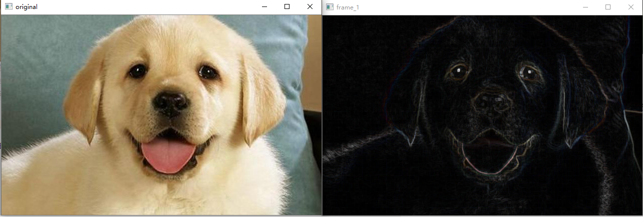
int main()
{
	Mat src = imread("path/to/img");
	if (src.empty())
	{
		cout << "no image" << endl;
		return 0;
	}
	Mat dst;
	Mat dst_dilate;
	Mat dst_erode;
	Mat RES;
	GaussianBlur(src, dst, Size(3, 3), 0.3);
	Mat kernel = getStructuringElement(MORPH_RECT, Size(3,3));
	dilate(dst, dst_dilate, kernel);
	erode(dst, dst_erode, kernel);
	RES = dst_dilate - dst_erode;

	namedWindow("original");
	imshow("original", src);

	namedWindow("frame_1");
	imshow("frame_1", RES);

	waitKey(0);

	return 1;
}

7.5 top hat and black hat operation

The top cap is the difference between the original image and the open operation. On the contrary, the black hat is the difference between the original image and the closing operation. After the opening operation, the cracks and local low brightness areas in the image are enlarged. This operation is often used to separate objects from the background. Black hat operation is used to separate patches darker than adjacent points.

The results of top hat and black hat operations are shown in the following two figures:


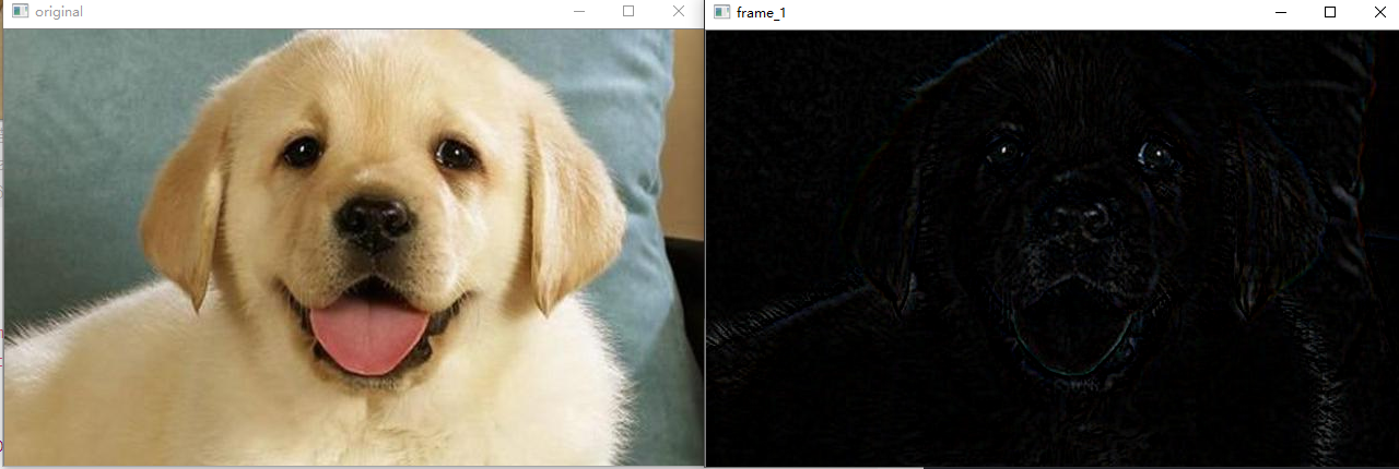
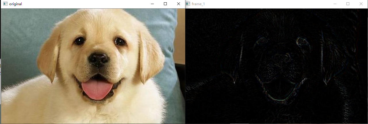
opencv can be used directly

morphologyEx(dst, dst_open, MORPH_BLACKHAT,kernel) // Black hat
//or
morphologyEx(dst, dst_open, MORPH_TOPHAT,kernel) // Top cap

You can also use the original figure to subtract the result after the open operation or the close operation.

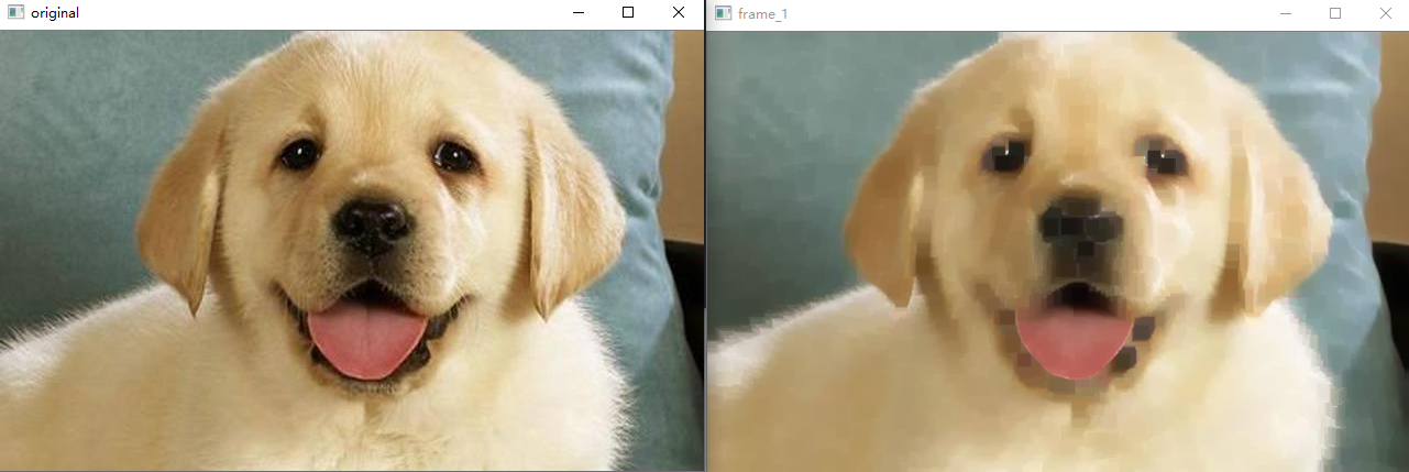
8. Image pyramid

The significance of graphic pyramid is to find the image features in different image spaces. Image pyramid makes the image features better preserved.
Generally, objects with very small size need to be observed with large resolution. On the contrary, if the size of the object is relatively large, only low resolution is enough. If you need to observe both small and large objects in a task, you need to use multi-resolution to observe. At this time, the image pyramid is born. The specific operation can be understood as up sampling and down sampling of the image. The image after down sampling is 1 / 2 of the width and height of the original image, and the image obtained by up sampling is twice that of the original image.
The specific implementation methods of up sampling and down sampling are as follows:

int main()
{
	Mat src = imread("2.jpeg");
	if (src.empty())
	{
		cout << "no image" << endl;
		return 0;
	}
	Mat RES;
	int cols, rows;
	cols = src.cols;
	rows = src.rows;
	
	//Up sampling
	pyrUp(src, RES, Size(cols * 2, rows * 2));  //Here can only be cols first and then rows, and can only be multiplied by twice, otherwise an error will be reported.
	//Down sampling
	pyrDown(src, RES, Size(cols / 2, rows / 2));
	
	
	namedWindow("original");
	imshow("original", src);

	namedWindow("frame_1");
	imshow("frame_1", RES);
	
	waitKey(0);
	
	return 1;
}

8.1 Gaussian pyramid

In a Gaussian pyramid, subsequent images are weighted down using a Gaussian average (Gaussian blur) and scaled down. Each pixel containing a local average corresponds to a neighborhood pixel on a lower level of the pyramid.

8.1.1 Gauss difference and its function

Difference of Gaussian - Dog:
Definition: subtract the results of Gaussian blur on the same image under different parameters to obtain the output image, which is called Gaussian difference. It is often used in gray image enhancement and corner detection.

Gauss's different steps can be understood this way.
1. First, a gray image is processed with Gaussian blur to obtain the processed image p1.
2. After processing P1 with Gaussian blur, P2 is obtained
3. When using p2 - p1, get the difference between the two.

8.2 Laplace pyramid

A Laplacian pyramid is very similar to a Gaussian pyramid but saves the difference image of the blurred versions between each levels. Only the smallest level is not a difference image to enable reconstruction of the high resolution image using the difference images on higher levels. This technique can be used in image compression.