Learn image gradients, image boundaries, etc.
The functions used are cv2.Sobel(), cv2.Schar(), cv2.Laplacian(), and so on.

principle

The_gradient is simply derivation, and OpenCV provides three different gradient filters, or high-pass filters: Sobel, Scharr, and Laplacian.Sobel, Scharr actually implements the first or second derivatives.Scharr is an optimization of Sobel when solving gradient angles using a small convolution kernel.Laplacian is the second derivative.

1. Sobel and Charr operators

The_Sobel operator is a combination of Gaussian smoothing and differential operation, so it has good noise resistance, can set the direction of derivation (xorder or yorder), and can also set the size of the convolution kernel used (ksize). If ksize=-1, a 3x3 Scharr filter will be used, which is more effective than a 3x3 Sobel.The filters are good (and the speeds are the same, so Scharr filters should be used whenever possible when using a 3x3 filter).The convolution kernel of the 3x3 Scharr filter is as follows: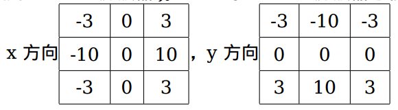

2. Laplacian Operator

Laplacian operators can be defined as second derivatives, assuming that their discrete implementation is similar to second-order Sobel derivatives. In fact, OpenCV directly calls Sobel operators when calculating Laplacian operators.The formula is as follows: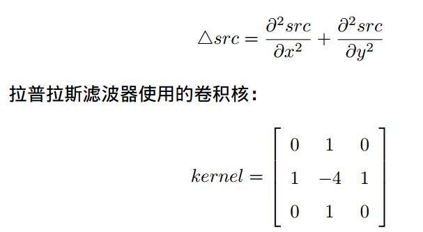

Code:

import cv2
import numpy as np 
from matplotlib import pyplot as plt 

img = cv2.imread('image/2.png',0)

laplacian = cv2.Laplacian(img, cv2.CV_64F)
sobelx = cv2.Sobel(img, cv2.CV_64F, 1, 0,ksize=5)
sobely = cv2.Sobel(img, cv2.CV_64F, 0, 1,ksize=5)
plt.subplot(2,2,1),plt.imshow(img,cmap='gray')
plt.title('Original'),plt.xticks([]),plt.yticks([])
plt.subplot(2,2,2),plt.imshow(laplacian,cmap='gray')
plt.title('Laplacian'),plt.xticks([]),plt.yticks([])
plt.subplot(2,2,3),plt.imshow(sobelx,cmap='gray')
plt.title('Sobel_X'),plt.xticks([]),plt.yticks([])
plt.subplot(2,2,4),plt.imshow(sobely,cmap='gray')
plt.title('Sobel_Y'),plt.xticks([]),plt.yticks([])
plt.show()

Result diagram: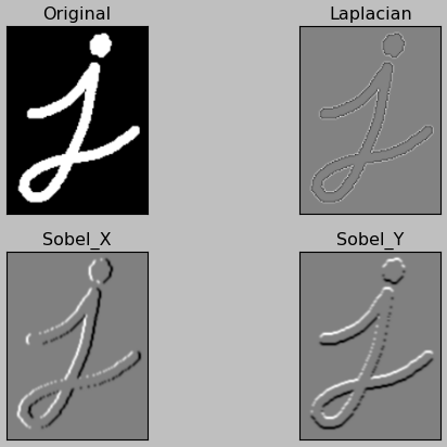

Note: The depth (data type) of the output image can be set by parameter -1 to be consistent with the original image, but cv2.CV_64F is used in the code. Why?Imagine that a black-to-white boundary derivative is an integer, and a white-to-black boundary point derivative is a negative number.If the depth of the original image is np.int8, all negative values will be truncated to zero, in other words, the boundary will be lost.So if you want to detect both boundaries, the best way is to set the output data type higher, such as cv2.CV_16S, cv2.CV_64F, and so on.Take the absolute value and turn it back to cv2.CV_8U.The following example demonstrates the different effects of different depths of the output picture.

import cv2
import numpy as np 
from matplotlib import pyplot as plt 

img = cv2.imread('image/4.png',0)
sobelx8u = cv2.Sobel(img, cv2.CV_8U, 1, 0,ksize=5)
sobelx64f = cv2.Sobel(img, cv2.CV_64F, 1, 0,ksize=5)
abs_sobel64f = np.absolute(sobelx64f)
sobel_8u = np.uint8(abs_sobel64f)
plt.subplot(1,3,1),plt.imshow(img,cmap='gray')
plt.title('Original'),plt.xticks([]),plt.yticks([])
plt.subplot(1,3,2),plt.imshow(sobelx8u,cmap='gray')
plt.title('Sobel CV_8U'),plt.xticks([]),plt.yticks([])
plt.subplot(1,3,3),plt.imshow(sobel_8u,cmap='gray')
plt.title('Sobel abs(CV_64F'),plt.xticks([]),plt.yticks([])
plt.show()

Result diagram: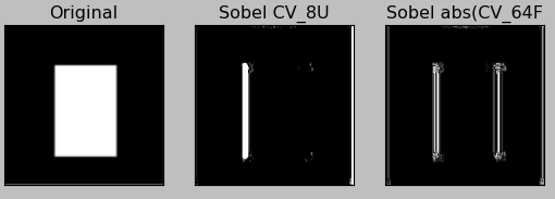

Reference: opencv Official Tutorial Chinese Edition (For Python)