1 image noise

Because the process of image acquisition, processing and transmission will inevitably be polluted by noise, which hinders people's understanding, analysis and processing of images. Common image noises include Gaussian noise, salt and pepper noise and so on.

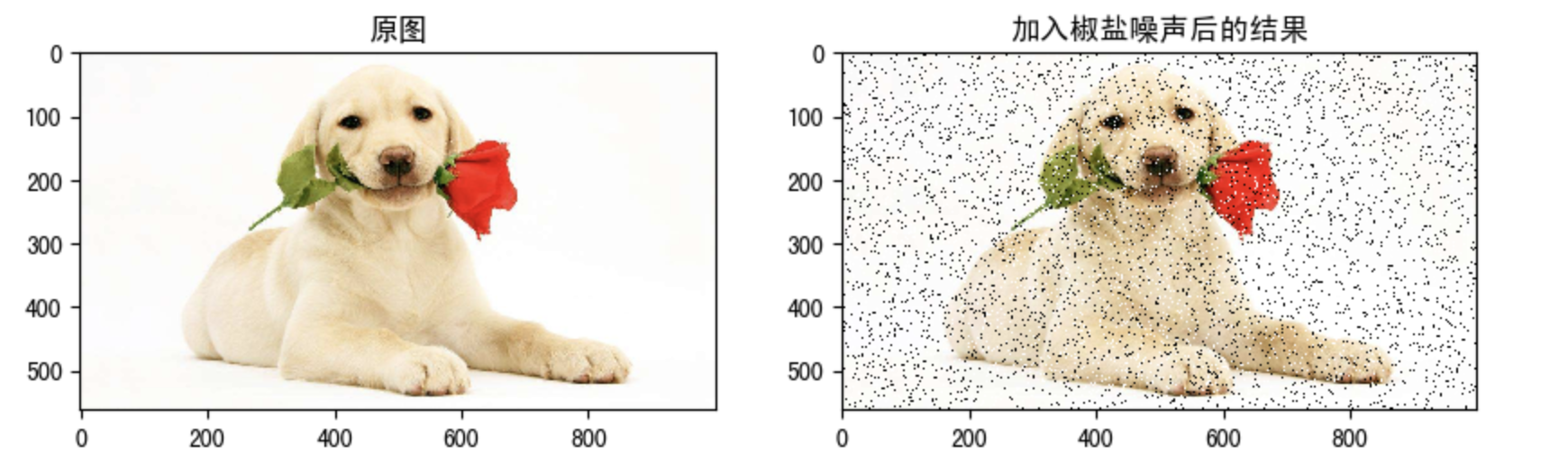
1.1 salt and pepper noise

Salt and pepper noise, also known as impulse noise, is a kind of noise often seen in images. It is a kind of random white or black spots. It may be that there are black pixels in bright areas or white pixels in dark areas (or both). Salt and pepper noise may be caused by sudden strong interference of image signal, analog-to-digital converter or bit transmission error. For example, a failed sensor causes the pixel value to be the minimum value, and a saturated sensor causes the pixel value to be the maximum value.

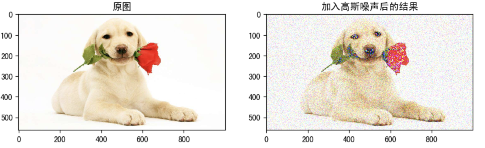
1.2 Gaussian noise

Gaussian noise is a kind of noise whose noise density function obeys Gaussian distribution. Due to the mathematical ease of Gaussian noise in space and frequency domain, this noise (also known as normal noise) model is often used in practice. The probability density function of Gaussian random variable z is given by the following formula:

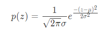
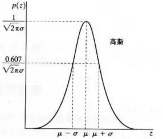
Where z represents the gray value, μ Represents the average or expected value of z, σ Represents the standard deviation of z. Square of standard deviation σ^ 2, called the variance of z. The curve of Gaussian function is shown in the figure.

2 Introduction to image smoothing

From the perspective of signal processing, image smoothing is to remove the high-frequency information and retain the low-frequency information. Therefore, we can implement low-pass filtering on the image. Low pass filtering can remove the noise in the image and smooth the image.

According to different filters, they can be divided into mean filter, Gaussian filter, median filter and bilateral filter.

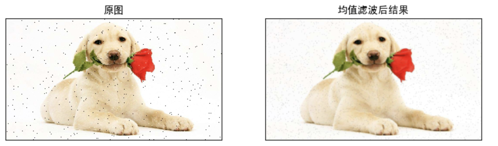
2.1 mean filtering

The mean filtering template is used to filter the image noise. Let Sxy indicate that the center is at point (x, y) and the dimension is m × The coordinate group of the rectangular sub image window of n. The mean filter can be expressed as:

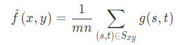
It is completed by a normalized convolution frame. It just replaces the central element with the average value of all pixels in the convolution frame coverage area.
The advantage of mean filtering is that the algorithm is simple and the calculation speed is fast. The disadvantage is that many details are removed while denoising, which makes the image blurred.

cv.blur(src, ksize, anchor, borderType)

Parameters:

src: input image 
ksize: Size of convolution kernel
anchor: Default value (-1,-1) ，Represents the nuclear center
borderType: Boundary type

Example:

import cv2 as cv
import numpy as np
from matplotlib import pyplot as plt
# 1 image reading
img = cv.imread('./image/dogsp.jpeg')
# 2-means filtering
blur = cv.blur(img,(5,5))
# 3 image display
plt.figure(figsize=(10,8),dpi=100)
plt.subplot(121),plt.imshow(img[:,:,::-1]),plt.title('Original drawing')
plt.xticks([]), plt.yticks([])
plt.subplot(122),plt.imshow(blur[:,:,::-1]),plt.title('Results after mean filtering')
plt.xticks([]), plt.yticks([])
plt.show()

2.2 Gaussian filtering

Two dimensional Gaussian filter is the basis of constructing Gaussian filter, and its probability distribution function is as follows:

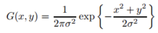
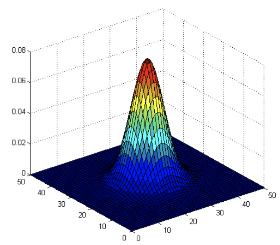Normal distribution is a bell curve. The closer it is to the center, the greater the value. The farther it is away from the center, the smaller the value. When calculating the smoothing result, you only need to take the "center point" as the origin and assign weights to other points according to their positions on the normal curve to obtain a weighted average.

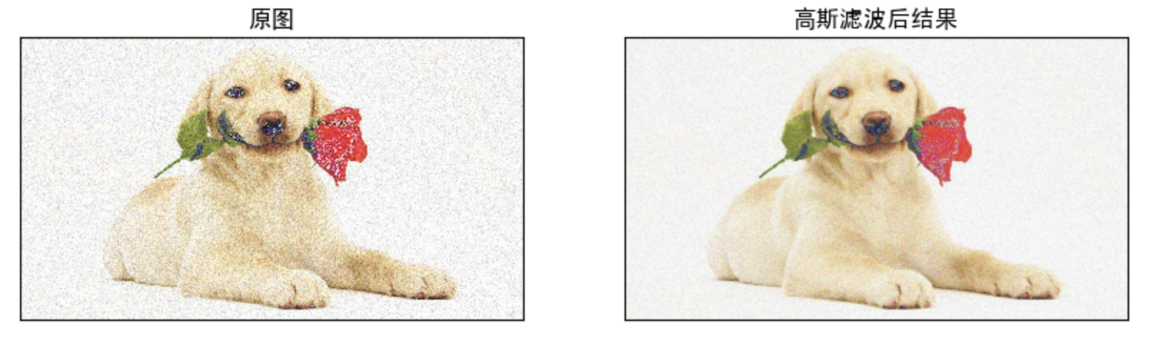
Gaussian smoothing is very effective in removing Gaussian noise from images.

Gaussian smoothing process:

Firstly, the weight matrix is determined
Assuming that the coordinates of the center point are (0,0), the coordinates of the 8 closest points are as follows:
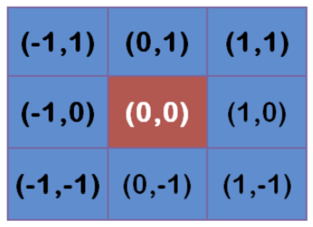Further points, and so on.

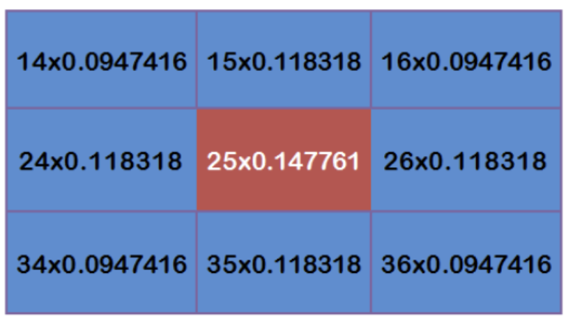
In order to calculate the weight matrix, you need to set σ Value of. assume σ= 1.5, the weight matrix with fuzzy radius of 1 is as follows:

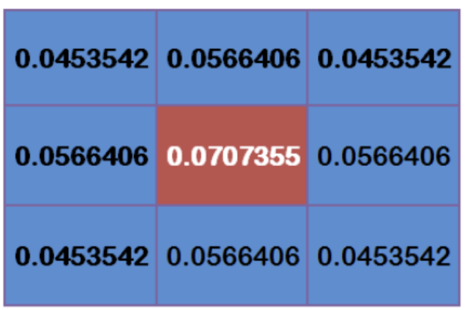
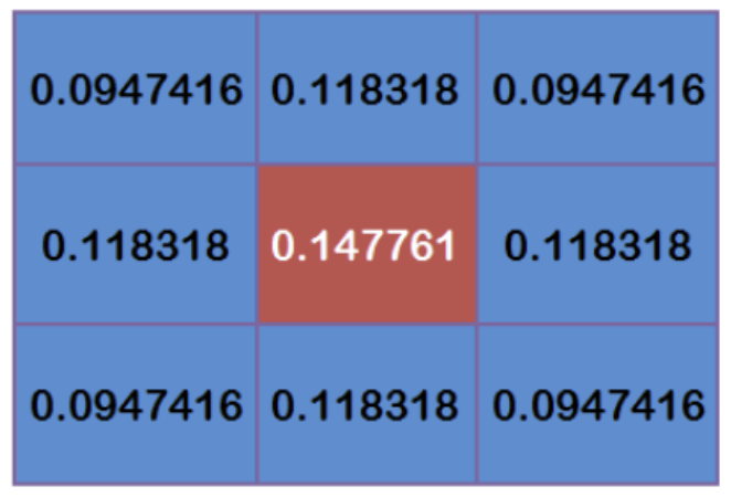
The total weight of these nine points is equal to 0.4787147. If only the weighted average of these nine points is calculated, the sum of their weights must be equal to 1. Therefore, the above nine values must be divided by 0.4787147 respectively to obtain the final weight matrix.

Calculate Gaussian blur
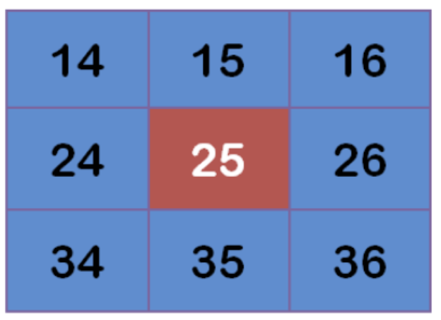
With the weight matrix, the value of Gaussian blur can be calculated.

Assuming that there are 9 pixels, the gray value (0-255) is as follows:

Multiply each point by the corresponding weight value:

obtain

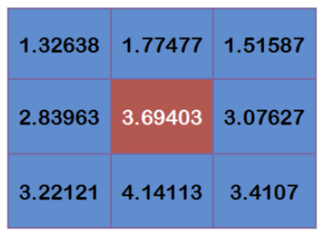
Add up these nine values to get the Gaussian blur value of the center point.

Repeat this process for all points to get the Gaussian blurred image. If the original image is a color image, Gaussian smoothing can be performed on the three RGB channels respectively.

cv2.GaussianBlur(src,ksize,sigmaX,sigmay,borderType)

Parameters:

src: input image 
ksize:The size of Gaussian convolution kernel. Note: the width and height of convolution kernel should be odd and can be different
sigmaX: Standard deviation in horizontal direction
sigmaY: The standard deviation in the vertical direction. The default value is 0, which means that it is consistent with sigmaX identical
borderType:Fill boundary type

Example:

import cv2 as cv
import numpy as np
from matplotlib import pyplot as plt
# 1 image reading
img = cv.imread('./image/dogGasuss.jpeg')
# 2 Gaussian filtering
blur = cv.GaussianBlur(img,(3,3),1)
# 3 image display
plt.figure(figsize=(10,8),dpi=100)
plt.subplot(121),plt.imshow(img[:,:,::-1]),plt.title('Original drawing')
plt.xticks([]), plt.yticks([])
plt.subplot(122),plt.imshow(blur[:,:,::-1]),plt.title('Results after Gaussian filtering')
plt.xticks([]), plt.yticks([])
plt.show()

2.3 median filtering

Median filtering is a typical nonlinear filtering technology. The basic idea is to replace the gray value of the pixel with the median of the gray value in the neighborhood of the pixel.

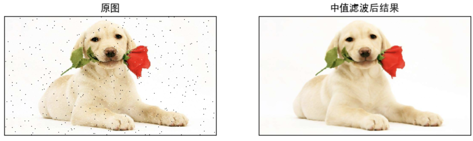
Median filtering is particularly useful for salt and pepper noise because it does not depend on the values in the neighborhood that are very different from the typical values.

cv.medianBlur(src, ksize )

Parameters:

src: input image 
ksize: Size of convolution kernel

Example:

import cv2 as cv
import numpy as np
from matplotlib import pyplot as plt
# 1 image reading
img = cv.imread('./image/dogsp.jpeg')
# 2-value filtering
blur = cv.medianBlur(img,5)
# 3 image display
plt.figure(figsize=(10,8),dpi=100)
plt.subplot(121),plt.imshow(img[:,:,::-1]),plt.title('Original drawing')
plt.xticks([]), plt.yticks([])
plt.subplot(122),plt.imshow(blur[:,:,::-1]),plt.title('Results after median filtering')
plt.xticks([]), plt.yticks([])
plt.show()

summary

Image noise

Salt and pepper noise: random white or black spots in an image
Gaussian noise: the probability density distribution of noise is normal

Image smoothing

Mean filtering: the algorithm is simple and the calculation speed is fast. While denoising, it removes many details and blurs the image

cv.blur()

Gaussian filtering: removing Gaussian noise

cv.GaussianBlur()

Median filtering: removing salt and pepper noise

cv.medianBlur()