K-nearest neighbor algorithm is one of the simplest machine learning algorithms. It is mainly used to divide objects into known classes and is widely used in life. For example, if a coach wants to select a group of long-distance runners, how to select them? He may use the k-nearest neighbor algorithm. He will choose those who are tall, long legs, light weight, small circumference of knee and ankle, obvious Achilles tendon and large foot arch as candidates. He will feel that such children have the potential of athletes, or that their characteristics are very close to those of athletes.

1. Theoretical basis

For example, it is known that A famous twin artist A and B look alike. If you want to judge whether the character on an image T is artist A or artist B, the specific steps of K-nearest neighbor algorithm are as follows:

1. Collect 100 photos of artist A and artist B.
2. Identify several important features used to identify the character and use these features to mark the photos of artist A and B. For example, according to A certain 4 characteristic, Each photo can be represented in the form of [156, 34, 890, 457] (i.e. A sample point). According to the above method, the data set FA of 100 photos of artist A and the data set FB of 100 photos of artist B are obtained. At this time, the elements in the data sets FA and FB are in the form of the above eigenvalues, and there are 100 such eigenvalues in each set. In short, the photos are represented by numerical values to obtain the numerical feature set of artist A (data set) numerical feature set FB of FA and artist B.
3. The feature of the image T to be recognized is calculated, and the feature value is used to represent the image T. For example, the eigenvalue TF of image T may be [257, 896, 236, 639].
4. Calculate the distance between the eigenvalue TF of image T and each eigenvalue in FA and FB.
5. Find out the sample points that produce K shortest distances (find the k nearest neighbors to T), count the number of sample points belonging to FA and FB in the K sample points, and determine T as the artist's image if there are more sample points in which dataset. For example, find 11 nearest points, among which 7 sample points belong to FA and 4 sample points belong to FB, then determine that the artist on this image T is A; On the contrary, if 6 of the 11 points belong to FB and 5 of them belong to FA, it is determined that the artist on this image T is B.

The above is the basic idea of K-nearest neighbor algorithm.

2. Calculation

The "feeling" of computer is realized through logical calculation and numerical calculation. Therefore, in most cases, we need to numerically process the objects to be processed by the computer and quantify them into specific values for subsequent processing. A typical method is to take some fixed features and quantify them.

After obtaining the eigenvalues of each sample, the k-nearest neighbor algorithm calculates the distance between the eigenvalues of the samples to be identified and the eigenvalues of the samples of each known classification, then finds out k nearest samples, and determines the classification of the samples to be identified according to the classification of the samples with the highest proportion among the k nearest samples.

2.1 normalization

Usually, due to the inconsistent dimensions of various parameters, it is necessary to process the parameters so that all parameters have equal weights.

In general, the parameters can be normalized. For normalization, the eigenvalue is usually divided by the maximum of all eigenvalues (or the difference between the maximum and the minimum).

2.2 distance calculation

Here, the Euclidean distance can be used to calculate the distance, that is, the square root of the sum of squares.

For example, there are eigenvalues A(185, 75) and B(175, 86) in the form of (height, weight). The distance between C(170, 80) and eigenvalues A and B is determined as follows:

• Distance between C and A:
  ( 185 − 170 ) 2 + ( 75 − 80 ) 2 {\sqrt{{{ \left( {185-170} \right) }\mathop{{}}\nolimits^{{2}}+{ \left( {75-80} \right) }\mathop{{}}\nolimits^{{2}}}}} (185−170)2+(75−80)2 ​
• Distance between C and B:
  ( 175 − 170 ) 2 + ( 86 − 80 ) 2 {\sqrt{{{ \left( {175-170} \right) }\mathop{{}}\nolimits^{{2}}+{ \left( {86-80} \right) }\mathop{{}}\nolimits^{{2}}}}} (175−170)2+(86−80)2 ​

3. Handwritten numeral recognition principle

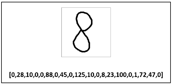
Suppose we want the program to recognize the number at the top of the figure below (of course, you know it is "8" at a glance, but now let the computer recognize it). The way of recognition is to successively calculate the distance between the digital image (i.e. the image with numbers written) and the digital image below, and which digital image is closest to it (at this time, k =1), it is considered to be the most similar image, so as to determine the number in the image.

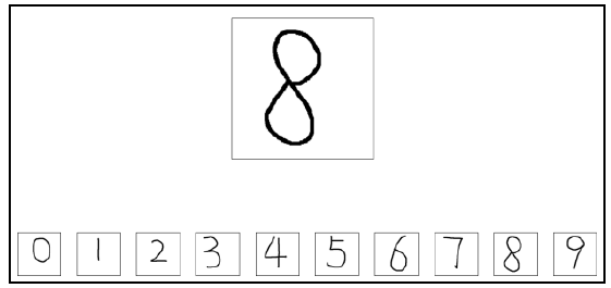
The following is an introduction from two aspects: eigenvalue extraction and number recognition.

3.1 eigenvalue extraction

Step 1: we divide the digital image into many small pieces, as shown in the figure below. Each number in the figure is divided into 5 rows and 4 columns, totaling 5 × 4 = 20 blocks. At this time, each small block is composed of many pixels. Of course, each pixel can also be understood as a smaller sub block.

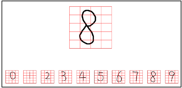
For the convenience of narration, these small blocks are represented as B (Bigger) and the pixels in B are recorded as S (Smaller). Therefore, the image of the number "8" to be recognized can be understood as:

• There are 5 rows and 4 columns in total × 4 = 20 small blocks B.
• Each small block B is actually composed of M × It is composed of N pixels (smaller block S). For the convenience of description, it is assumed that the size of each block is 10 × 10 = 100 pixels.

Step 2: calculate the number of black pixels in each block B. In other words, calculate how many smaller blocks S are black in each block B.

• The first small block B has 0 pixels in total (smaller block S) which are black and marked as 0.
• The second small block B has a total of 28 pixels (smaller block S) which are black and marked as 28.
• The third block B has a total of 10 pixels (smaller block S) which are black and marked as 10.
• The fourth block B has 0 pixels in total (smaller block S) which are black and marked as 0.

By analogy, calculate how many pixels in each small block B in the image with the number "8" are black.

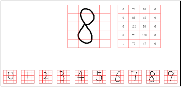
The number of black pixels in each small block B in different digital images is different. It is this difference that enables us to use this number (the number of black pixels in each block B) as a feature to represent each number.

Step 3: sometimes, for the convenience of processing, we will line up the obtained eigenvalues (written in array form).

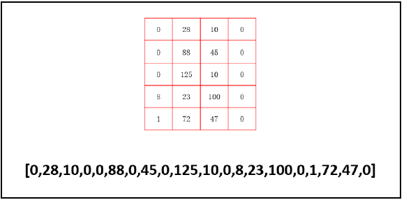
Of course, there is absolutely no need to do this in Python, because Python can easily directly process the data in the form of array at the top of the figure. Here, for the convenience of illustration, its eigenvalues are still processed as a line of numbers.

After the above processing, the eigenvalue of the digital "8" image becomes a line of numbers, as shown in the figure.

Step 4: similar to the image of the number "8", the eigenvalue of each digital image can be represented by a line of numbers. In a sense, this line number is similar to our ID number, which is generally unique.

3.2 digital identification

What digital recognition needs to do is to compare the image to be recognized with which image in the image set is the closest. Here, the nearest means the shortest Euclidean distance between them.

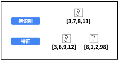
In this example, in order to facilitate explanation and understanding, the original lower 10 numbers are reduced to 2 (that is, the classification is reduced from 10 to 2). Assuming that the image to be recognized is the digital "8" image at the top of the figure, it is necessary to judge whether the image belongs to the classification of the digital "8" image at the bottom of the figure or the classification of the digital "7" image.

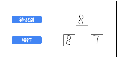
Step 1: extract the feature value, and extract the feature value of the image to be recognized and the feature value of the feature image respectively.

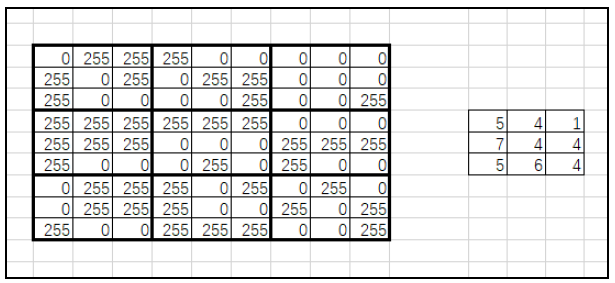
For the convenience of explanation and understanding, the features are simplified, and only 4 feature values (divided into 2) are extracted from each digital image × 2 = 4 sub blocks B), as shown. At this time, the extracted characteristic values are:

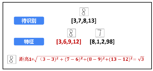
Step 2: calculate the distance between the image to be recognized and the feature image.

First, calculate the distance between the digital "8" image to be recognized and the digital "8" feature image below, as shown in the figure. Calculate the distance between the two:

Next, calculate the distance between the digital "8" image to be recognized and the digital "7" feature image, as shown in the figure. The distance between the two is:

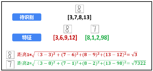
Step 3: identify.

According to the calculated distance, the digital "8" image to be recognized is closer to the digital "8" feature image. Therefore, the digital "8" image to be recognized is recognized as the digital "8" represented by the digital "8" feature image.

The k-nearest neighbor algorithm described above only considers the nearest neighbor, which is equivalent to the case of k =1 in k-nearest neighbor. In practice, in order to improve reliability, a large number of eigenvalues need to be selected. For example, 100 handwritten characters in different forms are selected for each number. For the 10 numbers 0 ~ 9, a total of 100 is required × 10 = 1000 characteristic images. When recognizing numbers, the distances between the digital images to be recognized and these feature images are calculated respectively. At this time, you can adjust K to a slightly larger value, such as k =11, and then see which feature images its nearest 11 neighbors belong to. For example, where:

• There are 8 digital "6" feature images.
• There are 2 digital "8" feature images.
• There is one characteristic image belonging to the number "9".

Through judgment, the number to be recognized is the number "6" represented by the digital "6" feature image.

3. User defined function handwritten numeral recognition

Opencv provides the function CV2 Kneasest() is used to implement the K-nearest neighbor algorithm, which can be called directly in OpenCV. In order to further understand the K-nearest neighbor algorithm and its implementation, this section first uses Python and OpenCV to implement an example of handwritten numeral recognition.

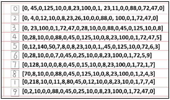
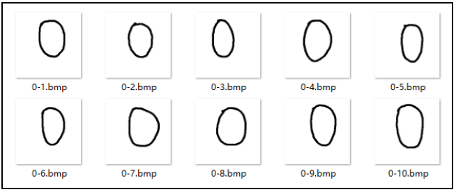
In this example, each number from 0 to 9 has 10 eigenvalues. For example, the characteristic value of the number "0" is shown in the figure. For ease of description, all these images used to judge classification are called feature images.

The following steps realize the recognition of handwritten digits.

3.1 data initialization

Initialize the data to be used in the program. The data involved mainly include path information, image size, number of eigenvalues, data used to store all eigenvalues, etc.

In this example:

• The feature image is stored in the "image" folder of the current path.
• There are 100 feature values (corresponding to 100 feature images) for judging classification.
• The number of rows (height) and the number of columns (width) of the feature image can be read through the program. You can also right-click the image and find the attribute value. Here, the set feature image set is used. Each feature image is 240 rows high and 240 columns wide.

Initialize the data to be used according to the above known conditions:

s='image\\' # The path where the image is located
num=100 # Number of common eigenvalues
row=240 # Number of rows of feature image
col=240 # Number of columns of feature image
a=np.zeros((num,row,col)) # a is used to store the values of all features

3.2 read characteristic image

This step reads all feature images into a. There are 10 numbers in total, and each number has 10 characteristic images, which are read by nested loop statements. The specific codes are as follows:

n=0 # n the number used to store the current image.
for i in range(0,10):
	for j in range(1,11):
		a[n,:,:]=cv2.imread(s+str(i)+'\\'+str(i)+'-'+str(j)+'.bmp',0)
		n=n+1

3.3 extracting feature values of feature images

When extracting feature values, the number of black pixels in each sub block and the number of white pixels in each sub block can be calculated. Here, we choose to calculate the number of white pixels (the pixel value is 255). According to the above idea, the relationship between image mapping and eigenvalue is shown in the figure.

It should be noted that the size of rows and columns of eigenvalues is 1 / 5 of the original image. Therefore, when designing the program, if the pixel at (row, col) in the original image is white, the value at (row/5, col/5) in the corresponding eigenvalue should be added by 1.

According to the above analysis, the code is written as follows:

feature=np.zeros((num,round(row/5),round(col/5))) # feature stores the characteristic values of all samples
#print(feature.shape) # If necessary, see what the shape of the feature looks like
#print(row) # If necessary, check the value of row and how many characteristic values (100) there are
for ni in range(0,num):
	for nr in range(0,row):
		for nc in range(0,col):
			if a[ni,nr,nc]==255:
				feature[ni,int(nr/5),int(nc/5)]+=1
f=feature #Simplified variable name

3.4 calculate the eigenvalue of the image to be recognized

Read the image to be recognized, and then calculate the eigenvalue of the image. The code is as follows:

o=cv2.imread('image\\test\\9.bmp',0) # Read the image to be recognized
# Read the value of the image
of=np.zeros((round(row/5),round(col/5))) # It is used to store the eigenvalues of the image to be recognized
for nr in range(0,row):
	for nc in range(0,col):
		if o[nr,nc]==255:
			of[int(nr/5),int(nc/5)]+=1

3.5 calculate the distance between the image to be recognized and the feature image

The distance between the image to be recognized and the feature image is calculated in turn. The code is as follows:

d=np.zeros(100)
for i in range(0,100):
	d[i]=np.sum((of-f[i,:,:])*(of-f[i,:,:]))

The array D is obtained by successively calculating the Euclidean distance between the feature value of the image to be recognized and each feature value in the data set F. The data set f sequentially stores the eigenvalues of a total of 100 feature images of numbers 0 ~ 9. Therefore, the index number in Array D corresponds to the number of each feature image. For example, d[mn] represents the distance between the image to be recognized and the nth feature image of the number "m". The corresponding relationship between the index of Array D and the feature image is shown in the table.

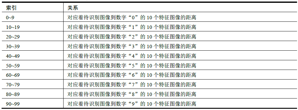
If you divide the index number by 10, the value obtained is exactly the number on its corresponding feature image. For example, d[34] corresponds to the Euclidean distance from the image to be recognized to the fourth feature image of the number "3". Divide 34 by 10 to get int(34/10) = 3, which is exactly the number on its corresponding feature image.

The relationship between the index and the feature image is determined. In the next step, the index can be calculated to achieve the purpose of digital recognition.

3.6 get k shortest distances and their indexes

Select k shortest distances from all the calculated distances, and calculate the index corresponding to the K shortest distances. The specific implementation methods are:

• Find the shortest distance (minimum) and its index (subscript) each time, and then replace the minimum value with the maximum value.
• Repeat the above process k times to obtain k indexes corresponding to the shortest distance.

The minimum value is replaced with the maximum value each time to ensure that the minimum value will not be found again in the next search for the minimum value. For example, find the values from small to large in the number sequence "11, 6, 3, 9".

• The minimum value "3" was found for the first time, and "3" was replaced with "11". At this time, the sequence to be searched becomes "11, 6, 11, 9".
• When looking for the minimum value for the second time, the minimum value found in the sequence "11, 6, 11, 9" is the number "6". At the same time, replace "6" with the maximum value "11" to obtain the sequence "11,11,11,9"

Repeat the above process continuously, and find the minimum value "9" for the third time and the minimum value "11" for the fourth time. Of course, in this example, the value is searched, and the index value is searched in the specific implementation.

d=d.tolist()
temp=[]
Inf = max(d)
#print(Inf)
k=7
for i in range(k):
	temp.append(d.index(min(d)))
	d[d.index(min(d))]=Inf

3.7 identification

According to the calculated index of k minimum values, combined with the above table, the number corresponding to the index can be determined. The specific implementation method is to divide the index value by 10 to get the corresponding number.

For example, when k =11, the indexes corresponding to the minimum 11 values are 66, 60, 65, 63, 68, 69, 67, 78, 89, 96 and 32. Their corresponding characteristic images are shown in the table.

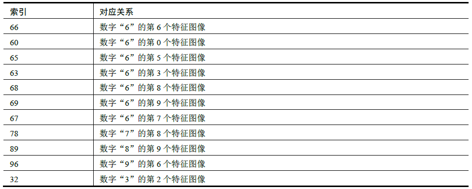
The above results show that seven of the feature images closest to the image to be recognized are the feature images of the number "6". Therefore, the image to be recognized is the number "6".

How to recognize numbers by program is discussed below. It is known that the number on the corresponding feature image can be obtained by dividing the index by 10. Therefore, for the above index division by 10:
(66, 60, 65, 63, 68, 69, 67, 78, 89, 96, 32) divide by 10 = (6, 6, 6, 6, 6, 6, 7, 8, 9, 3)

For the convenience of narration, the above division result is marked as dr. the number that appears most frequently in dr is the recognition result. For the above example, the number of "6" in dr is the largest, so the recognition result is the number "6".

Here, we use the index to determine which number appears the most in a group of numbers:

• Create an array r so that the initial value of its elements is 0.
• Take the number n from dr in turn, and add 1 to the value whose index position of array r is n. For example, the first number taken from dr is "6", add r[6] to 1; Take the second number from dr as "6", and add 1 to r[6]; By analogy, for dr = [6, 6, 6, 6, 6, 7, 8, 9, 3], the value of array r is [0, 0, 0, 1, 0, 0, 7, 1, 1, 1, 1].

In array r:

• r[0]=0, indicating that there is no element with value 0 in dr.
• r[3]=1, indicating that there is 1 "3" in dr.
• r[6]=7, indicating that there are 7 "6" in dr.
• r[7]=1, indicating that there is 1 "7" in dr.
• r[8]=1, indicating that there is 1 "8" in dr.
• r[9]=1, indicating that there is a "9" in dr.
• The remaining values in r are 0, indicating that the corresponding index does not exist in dr.

temp=[i/10 for i in temp]
# Array r is used to store results. r[0] represents the number of "0" in K-nearest neighbors, and r[n] represents the number of "n" in K-nearest neighbors
r=np.zeros(10)
for i in temp:
	r[int(i)]+=1
print('The current number may be:'+str(np.argmax(r)))

3.8 complete code

import cv2
import numpy as np
import matplotlib.pyplot as plt
# Read the value of the sample (characteristic) image
s='image\\' # Image path
num=100 # Total number of samples
row=240 # Number of rows of feature image
col=240 # Number of columns of feature image
a=np.zeros((num,row,col)) # Store values for all samples
#print(a.shape)
n=0 # Stores the number of the current image
for i in range(0,10):
	for j in range(1,11):
		a[n,:,:]=cv2.imread(s+str(i)+'\\'+str(i)+'-'+str(j)+'.bmp',0)
		n=n+1
#Feature extraction of sample image
feature=np.zeros((num,round(row/5),round(col/5))) # It is used to store the eigenvalues of all samples
#print(feature.shape) # Look at the shape of eigenvalues
#print(row) # Look at the value of row. How many eigenvalues are there (100)

for ni in range(0,num):
	for nr in range(0,row):
		for nc in range(0,col):
			if a[ni,nr,nc]==255:
				feature[ni,int(nr/5),int(nc/5)]+=1
f=feature # Simplified variable name
#####Calculate the eigenvalue of the current image to be recognized
o=cv2.imread('image\\test\\5.bmp',0) # Read the image to be recognized
##Read image value
of=np.zeros((round(row/5),round(col/5))) # Store the eigenvalue of the image to be recognized
for nr in range(0,row):
	for nc in range(0,col):
		if o[nr,nc]==255:
			of[int(nr/5),int(nc/5)]+=1
###Start the calculation, identify the number, calculate the number of the nearest numbers, and judge the result
d=np.zeros(100)
for i in range(0,100):
	d[i]=np.sum((of-f[i,:,:])*(of-f[i,:,:]))
#print(d)
d=d.tolist()
temp=[]
Inf = max(d)
#print(Inf)
k=7
for i in range(k):
	temp.append(d.index(min(d)))
	d[d.index(min(d))]=Inf
#print(temp) #See which eigenvalues are recognized
temp=[i/10 for i in temp]
# You can also return to array and use the function to process
#temp=np.array(temp)
#temp=np.trunc(temp/10)
#print(temp)
# Array r is used to store results. r[0] represents the number of "0" in K-nearest neighbors, and r[n] represents the number of "n" in K-nearest neighbors
r=np.zeros(10)
for i in temp:
	r[int(i)]+=1
#print(r)
print('The current number may be:'+str(np.argmax(r)))

4. Basic use of k-nearest neighbor module

In opencv, you don't need to write complex functions to implement the K-nearest neighbor algorithm, just call its own module functions directly. This section introduces how to use the K-nearest neighbor module of OpenCV through a simple example.

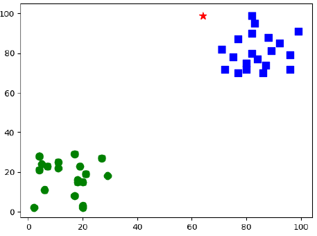
In this example, there are two sets of data sets for training located in different positions, as shown in the figure. Two data sets, one in the lower left corner; The other group is located in the upper right corner. Randomly generate a value, and use the K-nearest neighbor module in OpenCV to judge which group the random number belongs to.

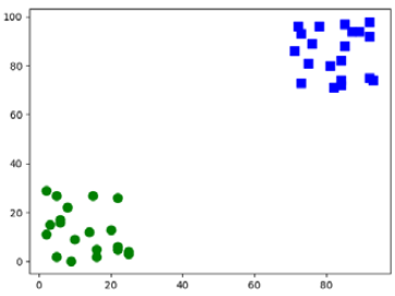
Among the above two groups of data, the x and y coordinate values of the data in the lower left corner are within the range of (0,30). The x and y coordinate values of the data in the upper right corner are within the range of (70, 100).

According to the above analysis, create two groups of data, each containing 20 pairs of random numbers (20 random data points):

rand1 = np.random.randint(0, 30, (20, 2)).astype(np.float32)
rand2 = np.random.randint(70, 100, (20, 2)).astype(np.float32)

• In the first group of random number rand1, the x and y coordinate values are located in the interval of (0,30).
• In the second group of random number rand2, the x and y coordinate values are located in the interval of (70, 100).

Next, assign labels to two sets of random numbers:

• Divide the first group of random number pairs into type 0 and label 0.
• Group 2 random number pairs are divided into type 1 and labeled 1.

Then, a pair of random number pairs with values within (0, 100) are generated:

test = np.random.randint(0, 100, (1, 2)).astype(np.float32)

Finally, use the K-nearest neighbor module of OpenCV to determine whether the generated random number pair test belongs to type 0 of rand1 or type 1 of rand2.

import cv2
import numpy as np
import matplotlib.pyplot as plt
# Data for training
# rand1 data at (0,30)
rand1 = np.random.randint(0, 30, (20, 2)).astype(np.float32)
# rand2 data is located at (70100)
rand2 = np.random.randint(70, 100, (20, 2)).astype(np.float32)
# rand1 and rand2 were spliced into training data
trainData = np.vstack((rand1, rand2))

# Data labels, of two types: 0 and 1
# r1Label corresponds to the label of rand1, which is of type 0
r1Label=np.zeros((20,1)).astype(np.float32)
# r2Label corresponds to the label of rand2, which is type 1
r2Label=np.ones((20,1)).astype(np.float32)
tdLable = np.vstack((r1Label, r2Label))

# Use green dimension type 0
g = trainData[tdLable.ravel() == 0]
plt.scatter(g[:,0], g[:,1], 80, 'g', 'o')
# Use blue to label type 1
b = trainData[tdLable.ravel() == 1]
plt.scatter(b[:,0], b[:,1], 80, 'b', 's')
# plt.show()

# Test is the random number used for the test, which is between 0 and 100
test = np.random.randint(0, 100, (1, 2)).astype(np.float32)
plt.scatter(test[:,0], test[:,1], 80, 'r', '*')

# Call the K-nearest neighbor module in OpenCV and train
knn = cv2.ml.KNearest_create()
knn.train(trainData, cv2.ml.ROW_SAMPLE, tdLable)
# Classification using K-nearest neighbor algorithm
ret, results, neighbours, dist = knn.findNearest(test, 5)
# Display processing results
print("The current random number can be determined as type:", results)
print("The five nearest neighbors to the current point are:", neighbours)
print("5 Distance between nearest neighbors: ", dist)
# You can observe the display and compare the above outputs
plt.show()

Run the above program, and the displayed running results (because they are random numbers, the results will be slightly different each time) are:

The current random number can be determined as type: [[1.]]
The five nearest neighbors to the current point are: [[1. 1. 1. 1. 1.]]
5 Distance between nearest neighbors: [[313. 324. 338. 377. 405.]]

At the same time, the program will also display the running results as shown in the figure. As can be seen from the figure, the random point (asterisk point) is closer to the point of the small square on the right (type 1), so it is determined to belong to type 1 of the small square.

5. Handwritten numeral recognition using OpenCV

This section uses the K-nearest neighbor module of OpenCV to recognize handwritten digits (the effect is very poor).

The effect is completely determined by the data set fed into the K-nearest neighbor function.

import cv2
import numpy as np
import matplotlib.pyplot as plt

#Read the value of the sample (characteristic) image
s='image\\'  #Image path
num=100 #Number of common samples
row=240 #Number of rows per digital image
col=240 #Number of columns per digital image
a=np.zeros((num,row,col)) #Used to store the values of all samples
#print(a.shape)
n=0 #The number used to store the current image.
for i in range(0,10):
    for j in range(1,11):
        a[n,:,:]=cv2.imread(s+str(i)+'\\'+str(i)+'-'+str(j)+'.bmp',0)
        n=n+1

#Feature extraction of sample image
feature=np.zeros((num,round(row/5),round(col/5))) #It is used to store the eigenvalues of all samples
#print(feature.shape)  #See what the shape of the feature looks like
#print(row)            #Look at the value of row. How many features (100) are there
for ni in range(0,num):
    for nr in range(0,row):
        for nc in range(0,col):
            if a[ni,nr,nc]==255:
                feature[ni,int(nr/5),int(nc/5)]+=1
f=feature   #Simplified variable name

#Process the feature as a single line
train = feature[:,:].reshape(-1,round(row/5)*round(col/5)).astype(np.float32) 
#print(train.shape)

#When labeling, it should be noted that range (0100) is not range (0101)
trainLabels = [int(i/10)  for i in range(0,100)]
trainLabels=np.asarray(trainLabels)
#print(*trainLabels)   #Print the test to see the label value

##Read image value
o=cv2.imread('image\\test\\5.bmp',0) #Read the image to be tested
of=np.zeros((round(row/5),round(col/5))) #It is used to store the eigenvalues of the test image
for nr in range(0,row):
    for nc in range(0,col):
        if o[nr,nc]==255:
            of[int(nr/5),int(nc/5)]+=1
test=of.reshape(-1,round(row/5)*round(col/5)).astype(np.float32) 

#Calling function identification
knn=cv2.ml.KNearest_create()
knn.train(train,cv2.ml.ROW_SAMPLE, trainLabels)
ret,result,neighbours,dist = knn.findNearest(test,k=5)
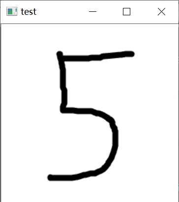
cv2.imshow("test",o)
print("The current random number can be determined as type:", result)
print("The five nearest neighbors to the current point are:", neighbours)
print("5 Distance between nearest neighbors: ", dist)
cv2.waitKey()
cv2.destroyWindow("test")

Run the above program, and the program running result is:

The current random number can be determined as type: [[5.]]
The five nearest neighbors to the current point are: [[5. 3. 5. 3. 5.]]
5 Distance between nearest neighbors: [[77185. 78375. 79073. 79948. 82151.]]