1, Introduction

Image processing can be divided into two parts, spatial domain (time domain) and frequency domain. Spatial domain is the direct pixel processing of the image, which can be divided into two ways: gray transformation and filtering. Gray change is to adjust the gray value of a single pixel, and filtering is for the whole image. Let's introduce the frequency domain. Here's a record and read a good blog post Explain Fourier transform in simple terms (really easy to understand)_ Blog of l494926429 - CSDN blog_ Fourier transform Have a basic understanding of Fourier transform. It can be said that Fourier transform transforms the original difficult time-domain signals into easy to analyze frequency-domain signals (signal spectrum). Some tools can be used to process and process these frequency-domain signals. Finally, the inverse Fourier transform can be used to convert these frequency domain signals into time domain signals.

In short, Fourier transform is to decompose an image into two parts: sinwt and coswt. These two parts correspond to the frequency domain, that is, an image is transformed from the spatial domain to the frequency domain, processed in the frequency domain, and then transferred to the spatial domain to form a closed loop. The value in the frequency domain is negative. Therefore, when displaying the transformation result, the real image and imaginary image are added together, which can also be in the form of amplitude image and phase image. The amplitude image contains most of the information needed in the original image, so only the amplitude image is usually used in the process of image processing. The purpose of Fourier transform is to carry out band-pass processing in the frequency domain, remove interference and obtain an ideal image, and then restore the image with inverse Fourier transform. Here, the restoration is not the original image, but the ideal target image. Therefore, we can use this technology to do image compression, steel scratch detection and other projects.

2, One dimensional mathematical derivation Fourier change

Any continuous periodic signal can be combined by a set of appropriate sinusoids (- - Genius said). In other words, any function can be approximated by the sum of infinitely many sins and cos. Although we don't know how Fourier himself thought of it, our later students still need to know why:

3, Two dimensional derivation

4, Fourier transform in OpenCV

Image Fourier transform dft of opencv learning (15)_ Yanyu blog - CSDN blog_ opencv Fourier transform

1. dft (Discrete Fourier transform)

void dft(
InputArray src, //The input image can be real or imaginary
OutputArray dst, // The size of the output image depends on the third parameter
int flags=0, // The default is 0 
      DFT_INVERSE: Replace the default forward transform with one-dimensional or two-dimensional inverse transform
      DFT_SCALE: Scaling scale identifier: calculate the scaling result according to the average number of data elements, if any N If there are multiple elements, the output result is expressed as 1/N Scaling output, often with DFT_INVERSE Use with
	  DFT_ROWS: Forward or reverse Fourier transform is performed on each row of the input matrix; This identifier can be used to reduce the cost of resources when processing a variety of appropriate, which are often complex operations such as three-dimensional or high-dimensional transformation
	  DFT_COMPLEX_OUTPUT: Forward transform one-dimensional or two-dimensional real arrays. Although the result is a complex array, it has the conjugate symmetry of the complex number. It can be filled with a real array with the same size as the original array. This is the fastest choice and the default method of the function. You may want to get a full-size complex array (such as simple spectral analysis, etc.). By setting the flag bit, the function can generate a full-size complex output array
      DFT_REAL_OUTPUT: The result of inverse transformation of one-dimensional and two-dimensional complex array is usually a complex matrix with the same size, but if the input matrix has conjugate symmetry of complex numbers (for example, a complex matrix with DFT_COMPLEX_OUTPUT The positive transformation result of the identifier) will output the real number matrix.
int nonzeroRows=0,The default is 0. When this parameter is not 0, the function will assume that there is only an input array (not set) DFT_INVERSE)The first row or the first output array of the DFT_INVERSE)Contains non-zero values. In this way, the function can process other rows more efficiently and save some time, especially when using this technology DFT It is very effective when calculating matrix convolution.
);

2. getOptimalDFTSize() gets the optimal width and height of dft transform

int getOptimalDFTSize(
int vecsize // Input vector size. DFT transform is not a monotonic function in a vector size. When calculating the convolution of two arrays or optical analysis of an array, it often expands some arrays with 0 to get a slightly larger array, so as to achieve the purpose of faster calculation than the original array. An array whose size is the second-order exponent (2,4,8,16,32...) has the fastest calculation speed. An array whose size is a multiple of 2, 3 and 5 (for example, 300 = 5 * 5 * 3 * 2 * 2) also has high processing efficiency.
getOptimalDFTSize()Function returns greater than or equal to vecsize Minimum value of N，The size is like this N Vector of DFT Transformation can get higher processing efficiency. At present N adopt p,q,r Wait for some integers N = 2^p*3^q*5^r.
This function cannot be used directly DCT(The optimal size of discrete cosine transform (DCT) can be estimated by getOptimalDFTSize((vecsize+1)/2)*2 Get.
)

 

#If 1 / / use of getoptimaldftsize

Mat  image_make_border(Mat &src) 
{
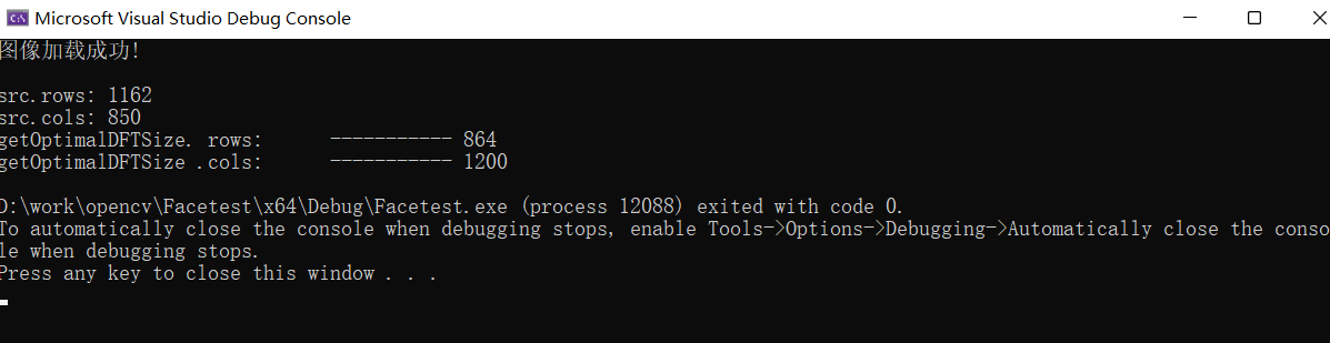
	cout << "src.rows: " << src.rows << endl;
	cout << "src.cols: " << src.cols << endl;

	int  w = getOptimalDFTSize(src.cols);  // The optimal width of DFT transform is obtained
	int  h = getOptimalDFTSize(src.rows);  // The optimal height of DFT transform is obtained

	cout << "getOptimalDFTSize. rows:      ----------- " << w << endl; 
	cout << "getOptimalDFTSize .cols:      ----------- " << h << endl; 

	Mat  p;
	//  Constant expands the boundary of the image up, down, left and right   
	copyMakeBorder(src, p, 0, h - src.rows, 0, w - src.cols, BORDER_CONSTANT, Scalar::all(0));

	p.convertTo(p,CV_32FC1);

	return p;

}
int main(int argc, char** argv)
{

	Mat src = imread("C:\\Users\\19473\\Desktop\\opencv_images\\602.png", IMREAD_GRAYSCALE);
	imshow("input image ", src);

	//Judge whether the image is loaded successfully
	if (src.empty())
	{
		cout << "Image loading failed!" << endl;
		return -1;
	}
	else
		cout << "Image loaded successfully!" << endl << endl;


	Mat  p = image_make_border(src);

	imshow("result: ", p / 255);


	waitKey(0);
	return 0;
}



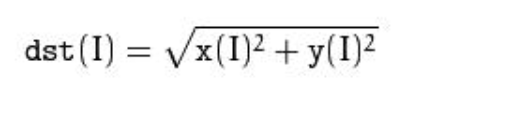
#endif

3.magnitude() calculates the amplitude of two-dimensional vector

void magnitude(
InputArray x, // The x-coordinate vector of floating-point data, that is, the real part we have long talked about
 InputArray y, //  The coordinates of y must be the same size as x
OutputArray magnitude  // The output is an output array of the same type and size as x
)；

4. The merge function is used to merge channels

merge(
const Mat* mv,  // Image matrix array
 size_t count,  // Number of matrices to be merged
 OutputArray dst  // 
)

5,split 

split(
	const cv::Mat& mtx, //input image 
	vector<Mat>& mv // Output multi-channel sequence (n single channel sequences)
)

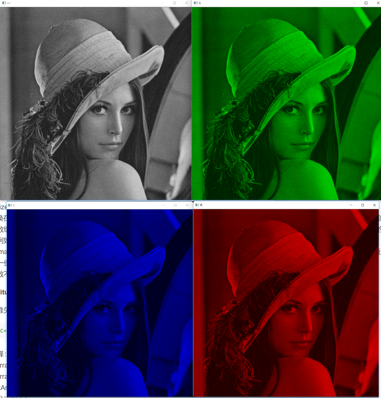
#If 1 / / image merging and splitting
int main()
{
	Mat src = imread("C:\\Users\\19473\\Desktop\\opencv_images\\601.png");
	imshow("src", src);

	//Apply for a three channel vector
	vector<Mat> rgbChannels(3);
	split(src, rgbChannels);

	//  Show different channels
	Mat blank_ch, fin_img;
	blank_ch = Mat::zeros(Size(src.cols, src.rows), CV_8UC1);

	// Showing Red Channel
	// G and B channels are kept as zero matrix for visual perception
	vector<Mat> channels_r;
	channels_r.push_back(blank_ch);
	channels_r.push_back(blank_ch);
	channels_r.push_back(rgbChannels[2]);

	/// Merge the three channels
	merge(channels_r, fin_img);
	imshow("R", fin_img);


	// Showing Green Channel
	vector<Mat> channels_g;
	channels_g.push_back(blank_ch);
	channels_g.push_back(rgbChannels[1]);
	channels_g.push_back(blank_ch);
	merge(channels_g, fin_img);
	imshow("G", fin_img);


	// Showing Blue Channel
	vector<Mat> channels_b;
	channels_b.push_back(rgbChannels[0]);
	channels_b.push_back(blank_ch);
	channels_b.push_back(blank_ch);
	merge(channels_b, fin_img);
	imshow("B", fin_img);

	waitKey(0);
	return 0;
}
#endif