Opencv Python Fourier transform

1, Image Fourier transform

Principle of two-dimensional Fourier transform

Gray image is composed of two-dimensional discrete points. Two dimensional discrete Fourier transform (2ddft) is often used in image processing. The spectrum of an image is obtained after Fourier transform. The frequency level in the spectrum indicates the intensity of gray level change in the image. The edge and noise in the image are often high-frequency signals, while the image background is often low-frequency signals. In the frequency domain, we can easily operate the high-frequency or low-frequency information of the image, and complete the operations of image denoising, image enhancement, image edge extraction and so on.

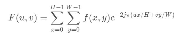
his in H , W branch other by chart image of high , wide , F ( u , v ) surface show frequency field chart image ， f ( x , y ) surface show Time field chart image ( some spot of image element ) ， u Model around by [ 0 , H − 1 ] , v Model around by [ 0 , W − 1 ] Where h and W are the height and width of the image respectively, F(u,v) represents the frequency domain image, f(x,y) represents the time domain image (pixels of a point), the range of u is [0, H-1], and the range of V is [0,W-1] Where h and W are the height and width of the image respectively, F(u,v) represents the frequency domain image, f(x,y) represents the time domain image (pixels of a point), the range of u is [0,H − 1], and the range of V is [0,W − 1]

Custom image Fourier transform function

1. Custom Fourier transform function

#Custom Fourier transform function
def dft(img):
    #Get image properties
    H,W,channel=img.shape
    #Define the frequency domain diagram. It can be seen from the formula that the result is complex, so it needs to be defined as complex matrix
    F = np.zeros((H, W,channel), dtype=np.complex)
    # Prepare a processing index corresponding to the original image position
    x = np.tile(np.arange(W), (H, 1))
    y = np.arange(H).repeat(W).reshape(H, -1)
    #Traversal by formula
    for c in range(channel):#Traverse the number of 3 channels of color
        for u in range(H):
            for v in range(W):
                F[u, v, c] = np.sum(img[..., c] * np.exp(-2j * np.pi * (x * u / W + y * v / H))) / np.sqrt(H * W)
    return F

2. Read the image, perform Fourier transform and display the transformed results

gray=cv2_imread("C://Users / / Xiaobai 2 / / Desktop//dd.png",1)
gray=cv2.resize(gray,(400,400))
img_dft = dft(gray)
dft_shift = np.fft.fftshift(img_dft)
fimg = np.log(np.abs(dft_shift))
cv2.imshow("fimg", fimg)
cv2.imshow("gray", gray)
cv2.waitKey(0)
cv2.destroyAllWindows()

Realization of Fourier transform with opencv library function

(1) Fourier transform function CV2 dft()

The function prototype is as follows:

img=cv2.dft(src, flags=None, nonzeroRows=None)

src indicates the input image, which needs to pass NP Float32 conversion format

Flag indicates the conversion flag, where CV2 DFT _ Invert performs reverse one-dimensional or two-dimensional conversion instead of the default forward conversion; cv2.DFT _SCALE represents the scaling result, divided by the number of array elements; cv2.DFT _ROWS performs forward or reverse transformation of each individual row of the input matrix. This flag can convert multiple vectors at the same time and can be used to reduce overhead to perform 3D and higher dimensional conversion, etc; cv2.DFT _COMPLEX_OUTPUT performs the forward conversion of 1D or 2D real number groups, which is the fastest choice and the default function; cv2.DFT _REAL_OUTPUT performs the inverse transformation of one-dimensional or two-dimensional complex array. The result is usually a complex array of the same size, but if the input array has conjugate complex symmetry, the output is a real array.

nonzeroRows means that when the parameter is not zero, the function assumes that only the first row of the nonzeroRows input array (not set) or only the first row of the output array (set) contains non-zero, so the function can process the remaining rows more efficiently and save some time; This technique is very useful for calculating array cross-correlation or using DFT convolution.

(2) Complex modulus function CV2 magnitude()

Since the output spectrum result is a complex number, cv2.0 needs to be called The magnitude() function converts the dual channel result of Fourier transform into the range of 0 to 255. The prototype of the function is as follows:

result=cv2.magnitude(x, y)

X represents the floating-point X coordinate value, that is, the real part

Y represents the floating-point y coordinate value, that is, the imaginary part

The final result is the modulus of the complex number

(3) Application examples

def cv2_imread(file_path, flag=1):
#Read picture data
    return cv2.imdecode(np.fromfile(file_path, dtype=np.uint8), flag)
gray=cv2_imread("C://Users / / Xiaobai 2 / / Desktop / / wallpaper 2 png",1)
gray=cv2.cvtColor(gray,cv2.COLOR_BGR2GRAY)
gray=cv2.resize(gray,(640,420))
np.float32(gray)
img_dft = cv2.dft(np.float32(gray),flags=cv2.DFT_COMPLEX_OUTPUT)
dft_shift = np.fft.fftshift(img_dft)
fimg = 20 * np.log(cv2.magnitude(dft_shift[:, :, 1], dft_shift[:, :, 0]))

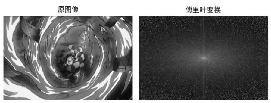
plt.subplot(121), plt.imshow(gray,'gray'), plt.title('Original image')
plt.axis('off')
plt.subplot(122), plt.imshow(np.int8(fimg),'gray'), plt.title('Fourier transform')
plt.axis('off')
plt.show()
cv2.waitKey(0)
cv2.destroyAllWindows()

Operation results:

2, Inverse Fourier transform of image

Principle of two-dimensional inverse Fourier transform

The principle of inverse Fourier transform is to restore the image frequency domain to the image time domain. The specific principle formula is as follows:

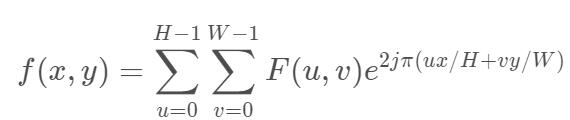
his in H , W branch other by chart image of high , wide , F ( u , v ) surface show frequency field chart image ， f ( x , y ) surface show Time field chart image ( some spot of image element ) ， x Model around by [ 0 , H − 1 ] , y Model around by [ 0 , W − 1 ] Where h and W are the height and width of the image respectively, F(u,v) represents the frequency domain image, f(x,y) represents the time domain image (the pixel of a point), the X range is [0, H-1], and the Y range is [0,W-1] Where h and W are the height and width of the image respectively, F(u,v) represents the frequency domain image, f(x,y) represents the time domain image (the pixel of a point), the X range is [0,H − 1], and the Y range is [0,W − 1]

Custom inverse Fourier transform function

The user-defined function is as follows:

def idft(G):
    H, W, channel = G.shape
    #Define blank time domain image
    out = np.zeros((H, W, channel), dtype=np.float32)
    # Prepare a processing index corresponding to the original image position
    x = np.tile(np.arange(W), (H, 1))
    y = np.arange(H).repeat(W).reshape(H, -1)
    #Traversal by formula
    for c in range(channel):
        for u in range(H):
            for v in range(W):
                out[u, v, c] = np.abs(np.sum(G[..., c] * np.exp(2j * np.pi * (x * u / W + y * v / H)))) / np.sqrt(W * H)
    # Tailoring
    out = np.clip(out, 0, 255)
    out = out.astype(np.uint8)
    return out

Implementation of inverse Fourier transform with OpenCV library function

(1) Inverse Fourier transform function

opencv can realize the function of inverse Fourier transform is CV2 Idft(), function prototype is as follows:

img=cv2.idft(src,flags,nonzeroRows)

src represents the input image, including real or complex numbers
flags indicates the conversion flag
nonzeroRows indicates the number of picture lines to be processed, and the contents of other lines are undefined

(2) Application examples

def cv2_imread(file_path, flag=1):
    # Read picture data
    return cv2.imdecode(np.fromfile(file_path, dtype=np.uint8), flag)


gray = cv2_imread("C://Users / / Xiaobai 2 / / Desktop / / wallpaper 2 png", 1)
gray = cv2.cvtColor(gray, cv2.COLOR_BGR2GRAY)
gray = cv2.resize(gray, (640, 420))

# Fourier transform
img_dft = cv2.dft(np.float32(gray), flags=cv2.DFT_COMPLEX_OUTPUT)
dft_shift = np.fft.fftshift(img_dft)# Move the frequency domain from the upper left corner to the middle
fimg = 20 * np.log(cv2.magnitude(dft_shift[:, :, 0], dft_shift[:, :, 1]))


# Inverse Fourier transform
idft_shift = np.fft.ifftshift(dft_shift)  # Move the frequency domain from the middle to the upper left corner
ifimg = cv2.idft(idft_shift)#Fourier library function call
ifimg = 20*np.log(cv2.magnitude(ifimg[:, :, 0], ifimg[:, :, 1]))#Convert to 0-255
ifimg=np.abs(ifimg)


# Draw picture
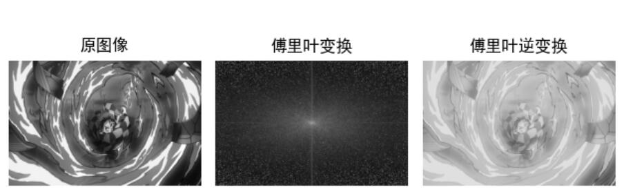
plt.subplot(131), plt.imshow(gray, 'gray'), plt.title('Original image')
plt.axis('off')
plt.subplot(132), plt.imshow(np.int8(fimg), 'gray'), plt.title('Fourier transform')
plt.axis('off')
plt.subplot(133), plt.imshow(np.int8(ifimg), 'gray'), plt.title('Inverse Fourier transform')
plt.show()
cv2.waitKey(0)
cv2.destroyAllWindows()

Operation results: