Simple threshold

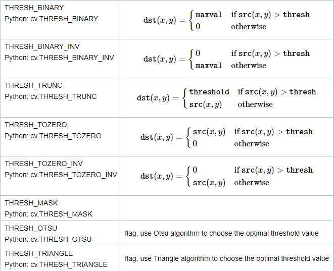
The same threshold is applied to each pixel. If the pixel value is less than the threshold value, set it to 0, otherwise set it to the maximum value. cv.threshold The function is used to set the threshold. The first parameter is the gray level image of the source image, the second parameter is the threshold used to classify the pixel values, and the third parameter is the maximum value allocated to the pixel values beyond the threshold. OpenCV provides different types of thresholds, which are given by the fourth parameter of the function.

Function:

retval, dst=cv.threshold(src, thresh, maxval, type[, dst]) uses a fixed threshold for each pixel

Parameters:

src	Input image, grayscale image (multi-channel, 8-bit or 32-bit floating point).
dst	Output arrays of the same size, type, and number of channels as src.
thresh	Threshold = Threshold = Threshold + Threshold + Threshold + Threshold + Threshold + Threshold + Threshold + Threshold + Threshold + Threshold + Threshold + Threshold + Threshold + Threshold + Threshold + Threshold + Threshold + Threshold
maxval	The value given when the pixel value exceeds (or is less than) the threshold, determined by type.
type	Threshold type (see) ThresholdTypes).

Return value:

retVal: Threshold used, used in Otsu's

dst: Threshold processed image

Threshold type:

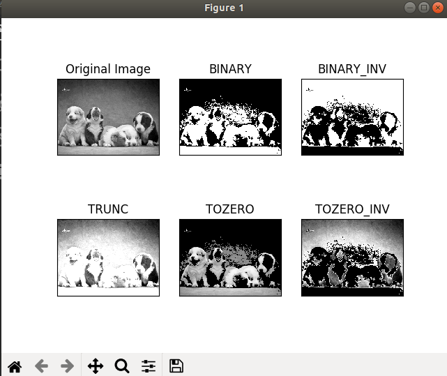
Give an example:

import cv2 as cv
import numpy as np
from matplotlib import pyplot as plt
img = cv.imread('4.jpg', 0)
ret, thresh1 = cv.threshold(img, 127, 255, cv.THRESH_BINARY)
ret, thresh2 = cv.threshold(img, 127, 255, cv.THRESH_BINARY_INV)
ret, thresh3 = cv.threshold(img, 127, 255, cv.THRESH_TRUNC)
ret, thresh4 = cv.threshold(img, 127, 255, cv.THRESH_TOZERO)
ret, thresh5 = cv.threshold(img, 127, 255, cv.THRESH_TOZERO_INV)
titles = ['Original Image', 'BINARY',
          'BINARY_INV', 'TRUNC', 'TOZERO', 'TOZERO_INV']
images = [img, thresh1, thresh2, thresh3, thresh4, thresh5]
for i in range(6):
    plt.subplot(2, 3, i+1), plt.imshow(images[i], 'gray')
    plt.title(titles[i])
    plt.xticks([]), plt.yticks([])
plt.show()

 

Adaptive threshold

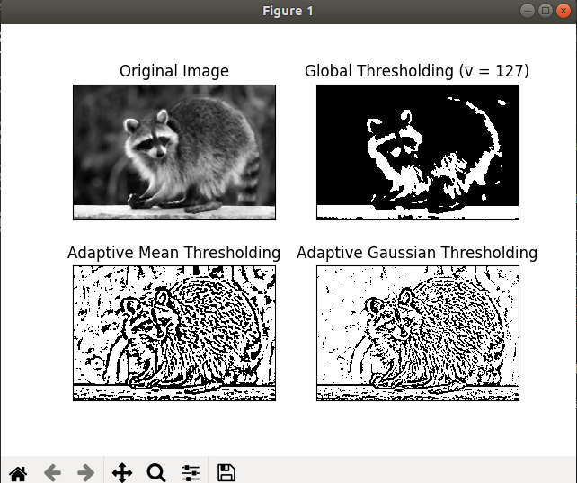
In the previous section, we used a global value as the threshold. But this does not apply to all cases, for example, if an image has different illumination conditions in different areas. In this case, the adaptive threshold can help, and the algorithm determines the threshold of the pixel according to the small area around the pixel. Therefore, for different regions of the same image, we get different thresholds, and for different illumination images, we get better results. In addition to the areas described above, cv.adaptiveThreshold The function also needs three other parameters.

function

dst=cv.adaptiveThreshold(src, maxValue, adaptiveMethod, thresholdType, blockSize, C[, dst])

Parameters:

src	Source 8-bit single channel image
dst	Target images of the same size and type as source images
maxValue	The value given when the pixel value exceeds (or is less than) the threshold, determined by type.
adaptiveMethod	The calculation method of threshold includes the following two types: see AdaptiveThresholdTypes.
thresholdType	The threshold type must be THRESH_BINARY or THRESH_BINARY_INV
blockSize	The size of the neighborhood of the pixel, which is used to calculate the threshold of the pixel: 3, 5, 7, and so on.
C	Constant Item in Threshold Calculating Method _

Among the above parameters, adaptiveMethod determines how the threshold is calculated.

　　cv.ADAPTIVE_THRESH_MEAN_C Threshold is the average value of neighborhood area minus constant C.

cv2.ADAPTIVE_THRESH_GAUSSIAN_C: Threshold is the Gauss weighted sum of neighborhood values minus constant C, and the weight is a Gauss window.

blockSize determines the size of neighborhood. C is a constant subtracted from the mean or weight of neighborhood pixels.

Give an example

import cv2 as cv
import numpy as np
from matplotlib import pyplot as plt
img = cv.imread('2.png',0)
# Median filter is used to suppress image noise. The edge of the signal can be protected from blurring while noise is filtered out.
img = cv.medianBlur(img,5)
# Simple threshold
ret,th1 = cv.threshold(img,127,255,cv.THRESH_BINARY)
# Adaptive threshold
th2 = cv.adaptiveThreshold(img,255,cv.ADAPTIVE_THRESH_MEAN_C,\
            cv.THRESH_BINARY,11,2)
th3 = cv.adaptiveThreshold(img,255,cv.ADAPTIVE_THRESH_GAUSSIAN_C,\
            cv.THRESH_BINARY,11,2)
titles = ['Original Image', 'Global Thresholding (v = 127)',
            'Adaptive Mean Thresholding', 'Adaptive Gaussian Thresholding']
images = [img, th1, th2, th3]
for i in range(4):
    plt.subplot(2,2,i+1),plt.imshow(images[i],'gray')
    plt.title(titles[i])
    plt.xticks([]),plt.yticks([])
plt.show()

 

 

Otsu's binarization

In global thresholding, we use an arbitrarily selected value as the threshold. Instead, Otsu's approach avoids having to select a value and automatically determine it.

Otsu's Binarization is a histogram-based binarization method, which needs to be used in conjunction with threshold function.

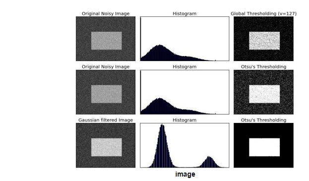
Consider images with only two different image values (bimodal images), where the histogram contains only two peaks. A good threshold should be in the middle of these two values (for non-bimodal images, the results obtained by this method may not be satisfactory). Similarly, Otsu's method determines an optimal global threshold from the image histogram.

To this end, use cv.threshold() Function, cv.THRESH_OTSU The most additional sign was introduced. Threshold can be chosen arbitrarily. Then, the algorithm finds an optimal threshold and the first output.

Look at the example below. The input image is a noisy image. In the first case, the global threshold of 127 is applied. In the second case, the threshold of Otsu is applied directly. In the third case, the image is filtered with 5x5 Gaussian kernel to remove noise, and then the Otsu threshold is applied. See how noise filtering improves the results.

 

import cv2 as cv
import numpy as np
from matplotlib import pyplot as plt
img = cv.imread('noisy2.png',0)
# global thresholding
ret1,th1 = cv.threshold(img,127,255,cv.THRESH_BINARY)
# Otsu's thresholding
ret2,th2 = cv.threshold(img,0,255,cv.THRESH_BINARY+cv.THRESH_OTSU)
# Otsu's thresholding after Gaussian filtering
blur = cv.GaussianBlur(img,(5,5),0)
# The threshold must be set to 0.
ret3,th3 = cv.threshold(blur,0,255,cv.THRESH_BINARY+cv.THRESH_OTSU)
# plot all the images and their histograms
images = [img, 0, th1,
          img, 0, th2,
          blur, 0, th3]
titles = ['Original Noisy Image','Histogram','Global Thresholding (v=127)',
          'Original Noisy Image','Histogram',"Otsu's Thresholding",
          'Gaussian filtered Image','Histogram',"Otsu's Thresholding"]
for i in xrange(3):
    plt.subplot(3,3,i*3+1),plt.imshow(images[i*3],'gray')
    plt.title(titles[i*3]), plt.xticks([]), plt.yticks([])
    plt.subplot(3,3,i*3+2),plt.hist(images[i*3].ravel(),256)
    plt.title(titles[i*3+1]), plt.xticks([]), plt.yticks([])
    plt.subplot(3,3,i*3+3),plt.imshow(images[i*3+2],'gray')
    plt.title(titles[i*3+2]), plt.xticks([]), plt.yticks([])
plt.show()

 

Otsu process:
1. Computing image histogram;
2. Setting a threshold, dividing the pixels whose histogram intensity is greater than the threshold into one group, and dividing the pixels whose intensity is less than the threshold into another group.
3. Calculate the migration numbers in the two groups and add them together.
4. Threshold 0-255 in order, repeat 1-3 steps until the minimum offset is obtained, and the corresponding value is the result threshold.