1, Background modeling

First, what belongs to the background? It's easy for us to judge which part of a picture is the background subjectively, but the computer can't identify which part is the background, so we have to find a way to tell the computer which part is the background.

1. Frame difference method

Because the target in the scene is moving, the image position of the target is different in different image frames. This kind of algorithm performs differential operation on two consecutive images in time, subtracts the corresponding pixels of different frames, and judges the absolute value of gray difference. When the absolute value exceeds a certain threshold, it can be judged as a moving target, so as to realize the target detection function.

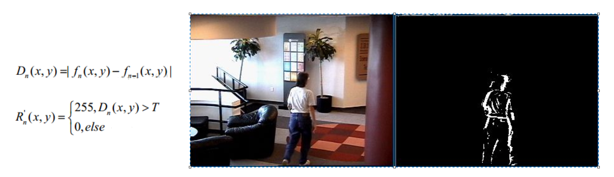
D formula is the judgment formula. Take the gray level of the next frame to subtract the gray level of the previous frame to judge the absolute value. Since the background is stationary, a general background can be obtained by performing multiple sets of calculations. However, we cannot guarantee that the video is absolutely still, so there may be some noise points in the calculated background.

2. Gaussian mixture model

Before foreground detection, the background is trained first, and a Gaussian mixture model is used to simulate each background in the image. The number of Gaussian mixtures in each background can be adaptive. Then, in the test phase, GMM matching is performed on the new pixels. If the pixel value can match one of the Gauss, it is considered as the background, otherwise it is considered as the foreground. Because the GMM model is constantly updated and learned in the whole process, it is robust to the dynamic background. Finally, through the foreground detection of a dynamic background with branch swing, good results are obtained.

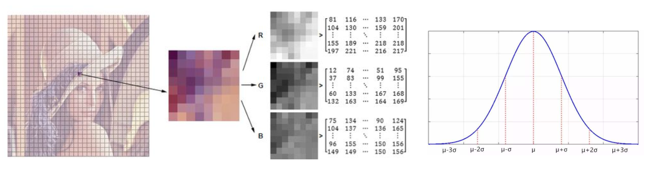
Gaussian distribution will give the general distribution range of a pixel, and judge in an interval. The result will be better than the previous method.
The actual distribution of the background should be a mixture of multiple Gaussian distributions, and each Gaussian model can also be weighted

Gaussian mixture model learning method

1. First, initialize each Gaussian model matrix parameter.

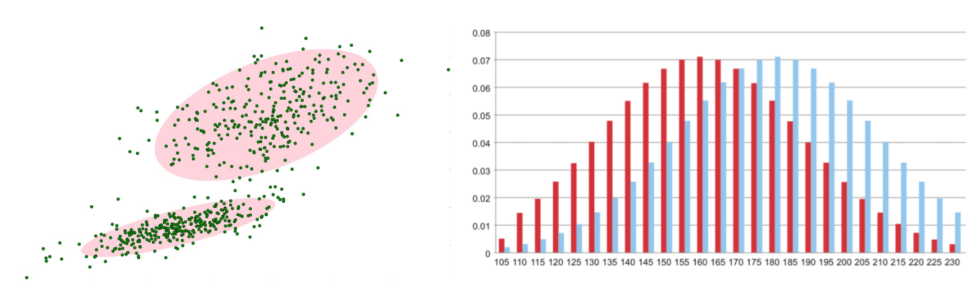
2. The T-frame data image in the video is used to train the Gaussian mixture model. The first pixel is used as the first Gaussian distribution.

3. When the later pixel value is compared with the previous Gaussian mean, if the difference between the pixel value and its model mean is within 3 times of variance, it belongs to the distribution, and its parameters are updated.

4. If the next pixel does not meet the current Gaussian distribution, use it to create a new Gaussian distribution.

Mixed Gaussian model test method

In the test stage, compare the value of the new pixel with each mean in the Gaussian mixture model. If the difference is between 2 times the variance, it is considered as the background, otherwise it is considered as the foreground. Assign 255 to the foreground and 0 to the background. In this way, a foreground binary map is formed.

3. Code

import numpy as np
import cv2

#Read test video
cap = cv2.VideoCapture('test.avi')
#Create morphological operation objects to facilitate contour finding
kernel = cv2.getStructuringElement(cv2.MORPH_ELLIPSE,(3,3))
#Create Gaussian mixture model for background modeling
fgbg = cv2.createBackgroundSubtractorMOG2()

while(True):
    ret, frame = cap.read()#Read frame by frame picture
    fgmask = fgbg.apply(frame)
    #Morphological operation to remove noise
    fgmask = cv2.morphologyEx(fgmask, cv2.MORPH_OPEN, kernel)
    #Find contours in video
    contours, hierarchy = cv2.findContours(fgmask, cv2.RETR_EXTERNAL, cv2.CHAIN_APPROX_SIMPLE)

    for c in contours:
        #Calculate the perimeter of each profile
        perimeter = cv2.arcLength(c,True)
        if perimeter > 188:
            x,y,w,h = cv2.boundingRect(c)
            #Draw this rectangle
            cv2.rectangle(frame,(x,y),(x+w,y+h),(0,255,0),2)    

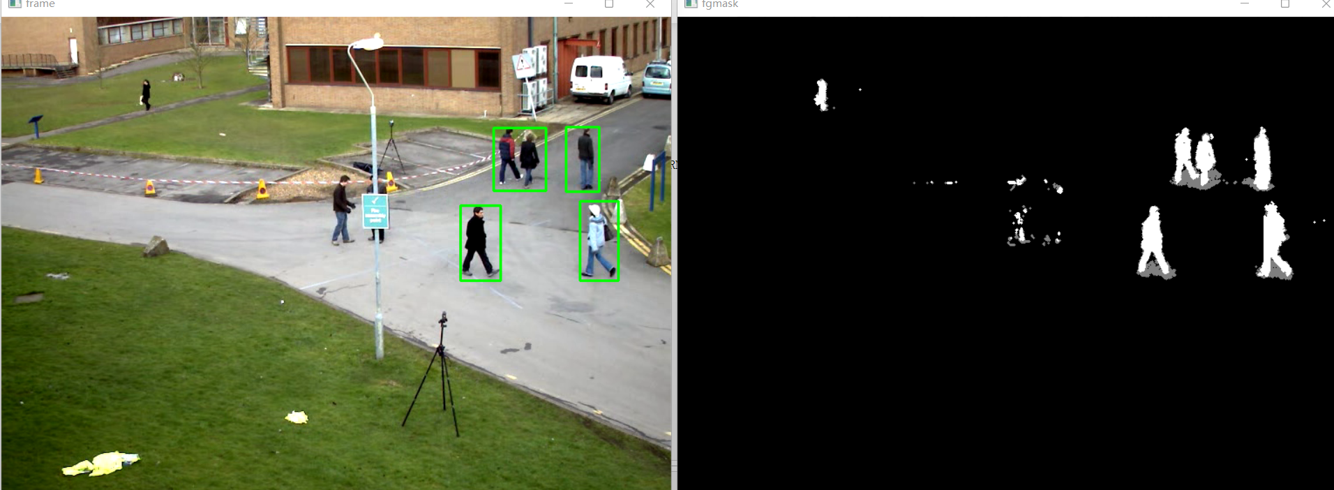
    cv2.imshow('frame',frame)
    cv2.imshow('fgmask', fgmask)
    k = cv2.waitKey(150) & 0xff
    if k == 27:
        break

cap.release()
cv2.destroyAllWindows()

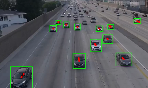
2, Optical flow estimation

Optical flow is the "instantaneous velocity" of the pixel motion of the space moving object on the observation imaging plane. According to the velocity vector characteristics of each pixel, the image can be dynamically analyzed, such as target tracking.

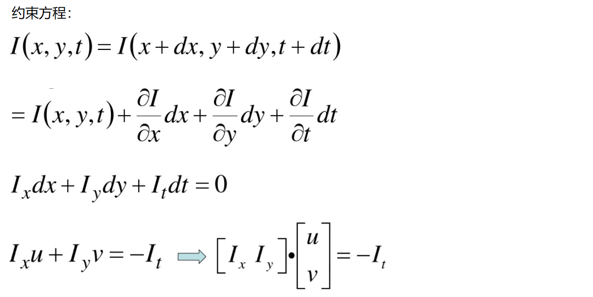
• Constant brightness: the brightness of the same point will not change with time.

• Small motion: the change of time will not cause drastic changes in position. Only in the case of small motion can the gray change caused by the change of unit position between the front and back frames be used to approximate the partial derivative of gray to position.

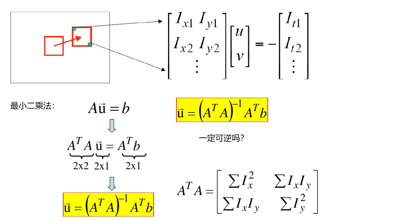
• Spatial consistency: adjacent points on a scene projected onto the image are also adjacent points, and the speed of adjacent points is consistent. Because there is only one constraint on the basic equation of the optical flow method, and the velocity in the x and y directions is required to have two unknown variables. Therefore, it is necessary to solve n multiple equations.

For example:

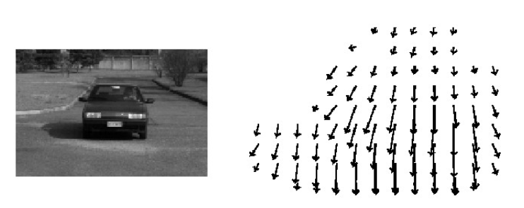
Our purpose is to determine the possible moving direction of each pixel to track the image target.

1. Lucas Kanade algorithm

Here we use the knowledge of calculus (I feel that we need to learn calculus again). First, we barely understand it as calculating the motion direction of each pixel in two coordinate directions.
Two unknowns cannot be solved by only one pixel.
We also need to find another feature to solve—— Corner

2.cv2.calcOpticalFlowPyrLK() method

Parameters:

   prevImage Previous frame image
   
   nextImage Current frame image
   
   prevPts Feature point vector to be tracked
   
   winSize Size of search window
   
   maxLevel Maximum pyramid layers

return:

nextPts Output tracking feature point vector

status Whether the feature point is found, the found status is 1, and the not found status is 0

The code is as follows (example):

import numpy as np
import cv2

cap = cv2.VideoCapture('test.avi')

# Parameters required for corner detection
feature_params = dict( maxCorners = 100,
                       qualityLevel = 0.3,
                       minDistance = 7)

# lucas kanade parameter
lk_params = dict( winSize  = (15,15),
                  maxLevel = 2)

# Random color bar
color = np.random.randint(0,255,(100,3))

# Get the first image
ret, old_frame = cap.read()
old_gray = cv2.cvtColor(old_frame, cv2.COLOR_BGR2GRAY)
# To return all detected feature points, you need to input the image, the maximum number of corners (efficiency), and quality factor (the larger the feature value, the better, to filter)
# The distance is equivalent to that there is something stronger than this corner in this interval, so don't use this weak one
p0 = cv2.goodFeaturesToTrack(old_gray, mask = None, **feature_params)

# Create a mask
mask = np.zeros_like(old_frame)

while(True):
    ret,frame = cap.read()
    frame_gray = cv2.cvtColor(frame, cv2.COLOR_BGR2GRAY)

    # The previous frame, the current image and the corner detected in the previous frame need to be passed in
    p1, st, err = cv2.calcOpticalFlowPyrLK(old_gray, frame_gray, p0, None, **lk_params)

    # st=1 indicates
    good_new = p1[st==1]
    good_old = p0[st==1]

    # Draw track
    for i,(new,old) in enumerate(zip(good_new,good_old)):
        a,b = new.ravel()
        c,d = old.ravel()
        mask = cv2.line(mask, (a,b),(c,d), color[i].tolist(), 2)
        frame = cv2.circle(frame,(a,b),5,color[i].tolist(),-1)
    img = cv2.add(frame,mask)

    cv2.imshow('frame',img)
    k = cv2.waitKey(150) & 0xff
    if k == 27:
        break

    # to update
    old_gray = frame_gray.copy()
    p0 = good_new.reshape(-1,1,2)

cv2.destroyAllWindows()
cap.release()