Other machine learning technologies: decision tree, anomaly detection, PCA

ID3: use the information entropy principle to select the attribute with the largest information gain as the classification attribute, recursively expand the branches of the decision tree, and complete the construction of the decision tree

Information Entropy: it is an index to measure the uncertainty of random variables. The greater the Entropy, the greater the uncertainty of variables

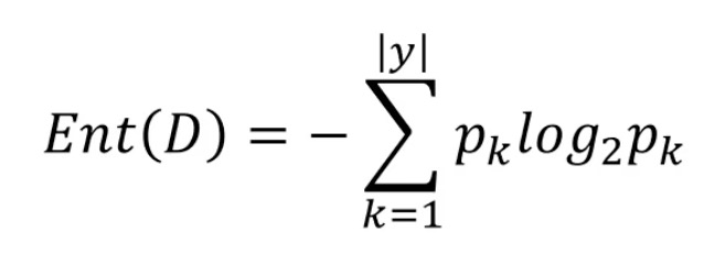D: the current sample set, Pk: the proportion of class k samples, such as 10 samples and 5 class 2 samples, with a proportion of 1 / 2

When Pk=1, i.e. 100% proportion, no uncertainty, Ent(D)=0

When Pk=0, that is, Pk=1 of another category, Ent(D)=0

Information gain: according to the information entropy, calculate the information gain brought by the sample division with attribute a (leaf), the greater the better

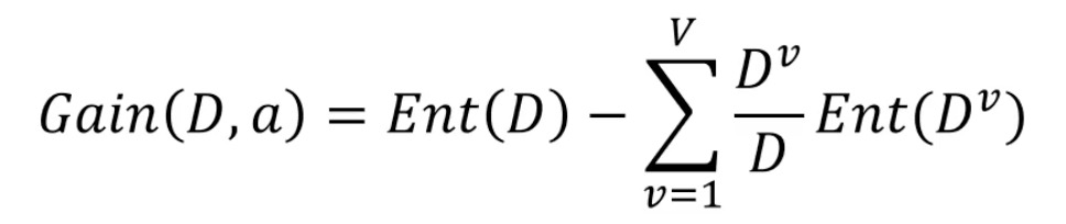Original information entropy - the information entropy after the new classification of attribute a, V: the number of categories divided according to attribute a, D: the total number of current samples, Dv: the number of samples of category v

Algorithm flow:

1. First, calculate the total information entropy Ent(D), that is, the proportion after classification

2. The information gain Gain(D,a) corresponding to each attribute is calculated in turn, and each attribute has two divisions (1 / 0)

3. The attribute with the largest information gain is the first node, and the second one is the second node

Advantages: it is possible to classify 10 samples with only 2 attributes, which is the advantage of maximizing information gain

2. Anomaly Detection

Anomaly detection: identify the data that does not meet the expected wear according to the input data

Probability density function: describes the possibility of random variables near a certain value point. Points with low probability density are abnormal points

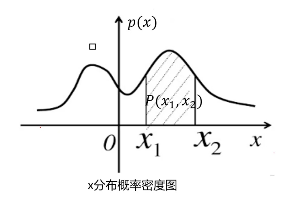
The probability of interval (x1,x2) is:

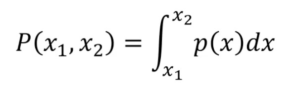That is, the area within the area

Gaussian distribution probability density function: obey normal distribution and bell curve

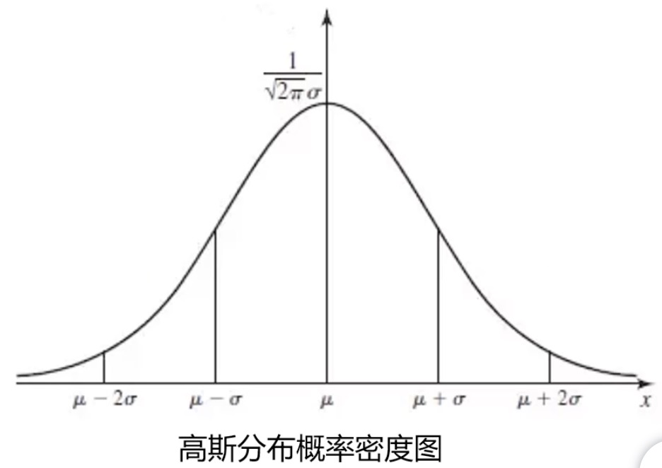
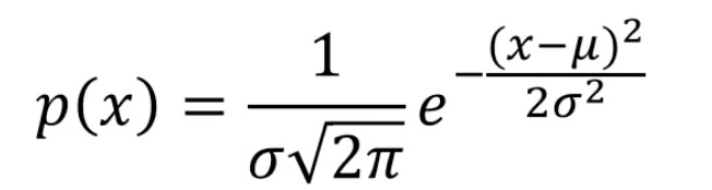Mean: mean, sigma: standard deviation

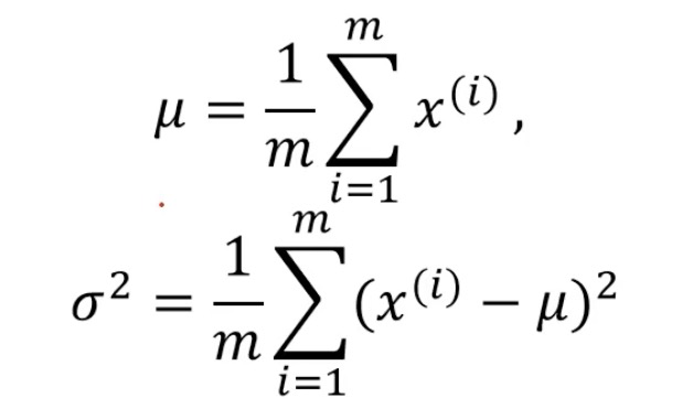mean: sum of all samples divided by the number of samples, sigma: sample distribution density (dispersion / concentration)

Algorithm flow:

Given the sample data xi, first calculate the mean and standard deviation
Then calculate the probability density p(x)
If P (x) < expected value empra, this point is an outlier

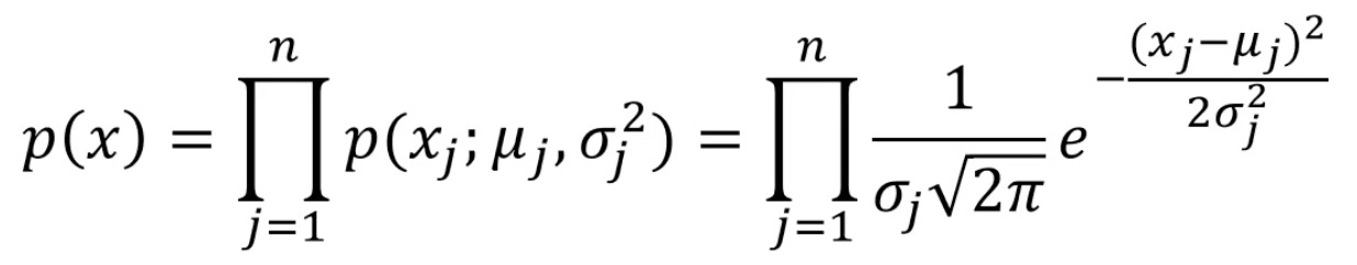
High dimensional Gaussian distribution probability density function:

3. Principal component analysis PCA

Data Dimensionality Reduction is realized by principal component analysis: the process of reducing the number of random variables and obtaining a group of irrelevant principal variables

Advantages: reduce the amount of data and improve efficiency. Low dimensional data can be visualized

Principal Component Analysis: find new data of K (k < n) dimension, make them reflect the main characteristics of things, and reduce the dimension under the condition of less information loss. For example, when the dimension 2 is reduced to the dimension 1, each point is projected onto the middle straight line, (when the dimension 3 is reduced to the dimension 2, the three-dimensional point is projected onto the plane). The projection represents Principal Component Analysis. The distance from each point to the projection straight line loses information, and the sum of loss information should be as small as possible

How to keep the main information: the larger the variance of the projected data, the more scattered (i.e. irrelevant) the different characteristic data after projection

Algorithm flow:

Raw data preprocessing (Standardization: mean=0, standard deviation sigma=1)
Calculate the eigenvector of covariance matrix and the variance of data after projection of each eigenvector
Determine the dimensionality reduction dimension k (with large variance) according to the requirements (task assignment or variance ratio)
The k-dimensional feature vector is selected to calculate the projection of data in its formation space

2, Code practice

1. Decision tree: Iris iris Iris data classification

Iris data set introduction: there are 3 categories, 150 records in total, and 50 data in each category. Each record has 4 characteristics, namely calyx length and width, petal length and width. 3 labels (0 / 1 / 2) represent 3 categories

'''
Task:
1. be based on iris_data.csv Data, establish decision tree model and evaluate model performance 
2. Visual decision tree structure 
3. modify min_samples_leaf Parameters, compare model results
'''

# 1. Load data
# load the data
import pandas as pd
import numpy as np
data = pd.read_csv('iris_data.csv')
data.head()

# 2. Assignment data
# define the X and y
X = data.drop(['target','label'],axis=1)
y = data.loc[:,'label']
print(X.shape,y.shape)

# 3. Establish decision tree model
# establish the decision tree model
from sklearn import tree
dc_tree = tree.DecisionTreeClassifier(criterion='entropy',min_samples_leaf=5)
dc_tree.fit(X,y)

# 3. Evaluate model performance
# evaluate the model
y_predict = dc_tree.predict(X)
from sklearn.metrics import accuracy_score
accuracy = accuracy_score(y,y_predict)
print(accuracy)

# 4. Visual decision tree
# visualize the tree
%matplotlib inline
from matplotlib import pyplot as plt
fig = plt.figure(figsize=(20,20))
tree.plot_tree(dc_tree,filled='True',feature_names=['SepalLength', 'SepalWidth', 'PetalLength', 'PetalWidth'],class_names=['setosa','versicolor','virginica'])

# 5. Modify the branch depth, that is, modify the min_samples_leaf parameter to compare the model results
dc_tree = tree.DecisionTreeClassifier(criterion='entropy',min_samples_leaf=1)
dc_tree.fit(X,y)
fig = plt.figure(figsize=(20,20))
tree.plot_tree(dc_tree,filled='True',feature_names=['SepalLength', 'SepalWidth', 'PetalLength', 'PetalWidth'],class_names=['setosa','versicolor','virginica'])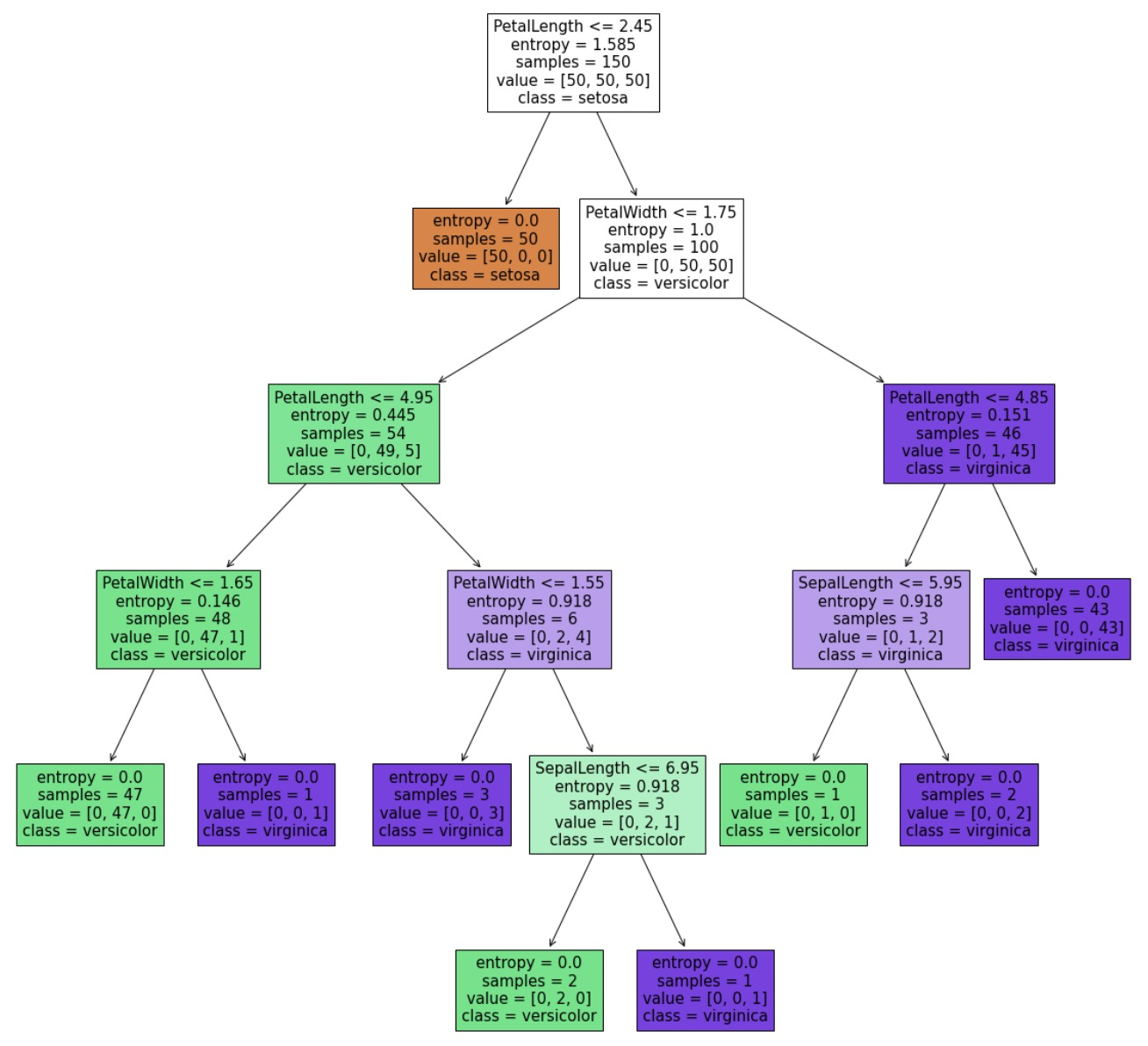

2. Anomaly detection

'''
load anomaly_data.csv Data, visual data distribution
'''
# 1. Load data
#load the data
import pandas as pd
import numpy as np
data = pd.read_csv('anomaly_data.csv')
data.head()

# 2. Data assignment, for convenience of calling
#define x1 and x2
x1 = data.loc[:,'x1']
x2 = data.loc[:,'x2']

# 3. Visual raw data: scatter diagram
#visualize the data
%matplotlib inline
from matplotlib import pyplot as plt
fig1 = plt.figure(figsize=(10,5)) # largeness of the shape of the figure
plt.scatter(x1,x2) # Data after calling assignment
plt.title('data')
plt.xlabel('x1')
plt.ylabel('x2')
plt.show()

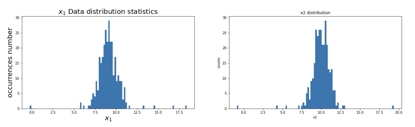
# 4. Visual data: draw the data distribution with histogram
# coding:utf-8
import matplotlib as mlp
font2 = {'family' : 'SimHei',
'weight' : 'normal',
'size'   : 20,
}
mlp.rcParams['font.family'] = 'SimHei'
mlp.rcParams['axes.unicode_minus'] = False

fig2 = plt.figure(figsize=(20,5))

plt.subplot(121)
plt.hist(x1,bins=100) # The data distribution is divided into 100 data segmentation and histogram visualization
plt.title('$x_1$ Data distribution statistics',font2)
plt.xlabel('$x_1$',font2)
plt.ylabel('occurrences number',font2)

plt.subplot(122)
plt.hist(x2,bins=100)
plt.title('x2 distribution')
plt.xlabel('x2')
plt.ylabel('counts')

plt.show()

fig1:

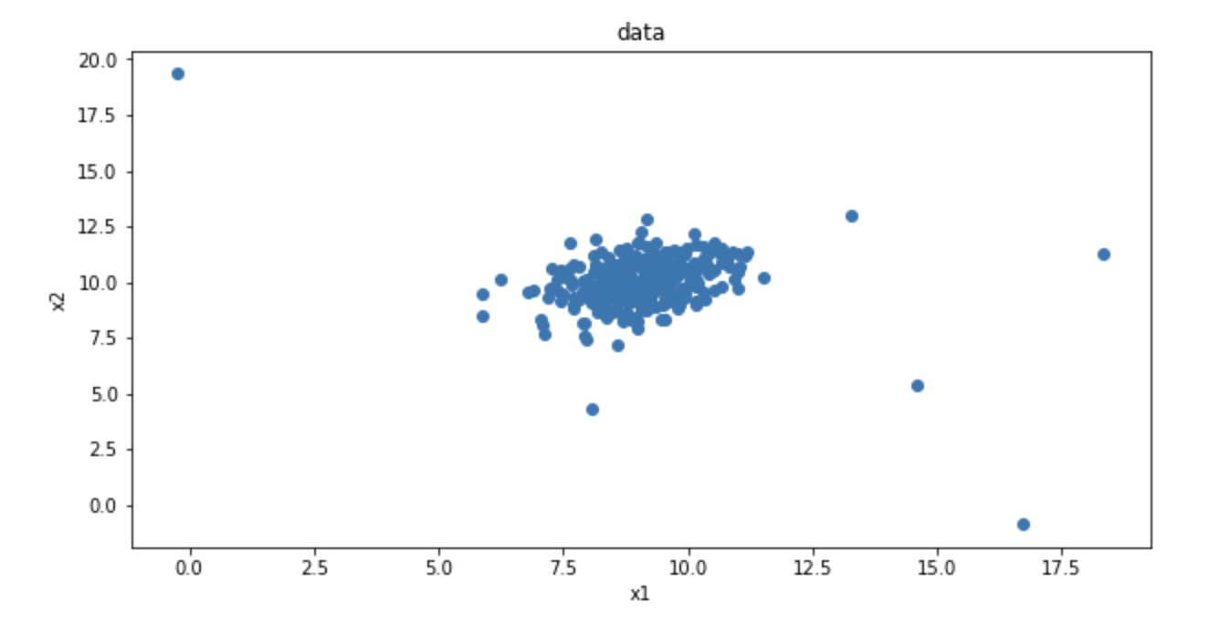
fig2:

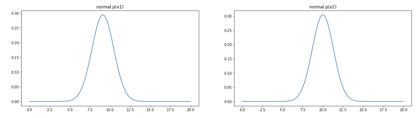
2.1} visualize the probability density function of Gaussian distribution

'''
Task 1:
Visual probability density function of Gaussian distribution 
'''
# 5. Calculate the mean and standard deviation
#calculate the mean and sigma of x1 and x2
x1_mean = x1.mean() # mean value
x1_sigma = x1.std() # standard deviation
x2_mean = x2.mean()
x2_sigma = x2.std()
print(x1_mean,x1_sigma,x2_mean,x2_sigma)

# 6. Calculate the probability density of Gaussian distribution
#calculate the gaussian distribution p(x)
from scipy.stats import norm

x1_range = np.linspace(0,20,300) # Generate 300 equally divided data points between 0 and 20
x1_normal = norm.pdf(x1_range,x1_mean,x1_sigma) # The corresponding Gaussian distribution probability density function of 300 data is calculated

x2_range = np.linspace(0,20,300)
x2_normal = norm.pdf(x2_range,x2_mean,x2_sigma)

# 7. Visualize the Gaussian distribution probability density curve, normal distribution, corresponding to the data distribution of x1 and x2
#visualize the p(x)
fig3 = plt.figure(figsize=(20,5)) # Create a new drawing object

plt.subplot(121) # 
plt.plot(x1_range,x1_normal)
plt.title('normal p(x1)')

plt.subplot(122)
plt.plot(x2_range,x2_normal)
plt.title('normal p(x2)')

plt.show()

fig3:

2.2} establish a model to realize the prediction of abnormal data points, visualize the abnormal detection and processing results, modify the content in the probability distribution threshold ellipticenvelope (content = 0.1), and view the impact of threshold change on the results

'''
Task 2:
The model is established to realize the prediction of abnormal data points, visualize the abnormal detection and processing results, and modify the probability distribution threshold EllipticEnvelope(contamination=0.1)Medium contamination，View the impact of threshold changes on the results
'''

# 1. Modeling of abnormal data points
#establish the model and predict
from sklearn.covariance import EllipticEnvelope
ad_model = EllipticEnvelope(contamination=0.03) # The probability density of each dimension is multiplied to obtain a threshold. When the threshold is large, it is easy to judge the normal point as an abnormal point
ad_model.fit(data)

# 2. Prediction abnormal data model
#make prediction
y_predict = ad_model.predict(data)
print(y_predict, pd.value_counts(y_predict))


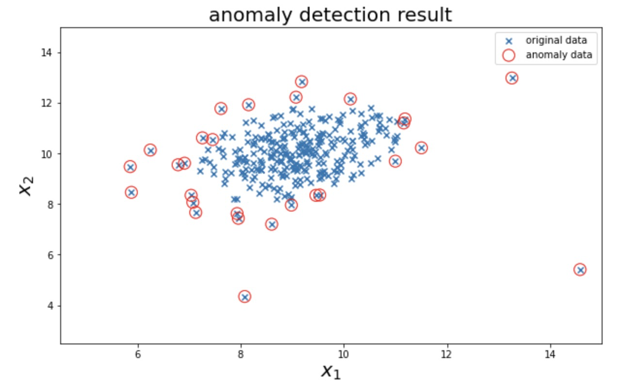
# 3. Visualize abnormal data
#visualize the result
fig4 = plt.figure(figsize=(10,6))
orginal_data=plt.scatter(data.loc[:,'x1'],data.loc[:,'x2'],marker='x')
anomaly_data=plt.scatter(data.loc[:,'x1'][y_predict==-1],data.loc[:,'x2'][y_predict==-1],marker='o',facecolor='none',edgecolor='red',s=150)

plt.title('anomaly detection result',font2) # Automatically find abnormal data
plt.xlabel('$x_1$',font2)
plt.ylabel('$x_2$',font2)
plt.legend((orginal_data,anomaly_data),('original data','anomaly data'))
plt.axis([4.5,15,2.5,15])
plt.show()

fig4:

3. Principal component analysis PCA: Iris dataset dimensionality reduction classification 4D - > 2D

# 1. load data
import pandas as pd
import numpy as np
data = pd.read_csv('/iris_data.csv')
data.head()

# 2. define X and y
X = data.drop(['target','label'],axis=1)
y = data.loc[:,'label']
y.head()

3.1} based on iris_data.csv data, establish KNN model to realize data classification (n_neighbors=3)

'''
Task 1:
be based on iris_data.csv Data, establishing KNN Model implementation data classification( n_neighbors=3) 
'''
# 3. Establish model, predict and calculate accuracy
#establish knn model and calculate the accuracy
from sklearn.neighbors import KNeighborsClassifier
KNN = KNeighborsClassifier(n_neighbors=3)
KNN.fit(X,y)

y_predict = KNN.predict(X)

from sklearn.metrics import accuracy_score
accuracy = accuracy_score(y,y_predict)
print(accuracy) # 0.96

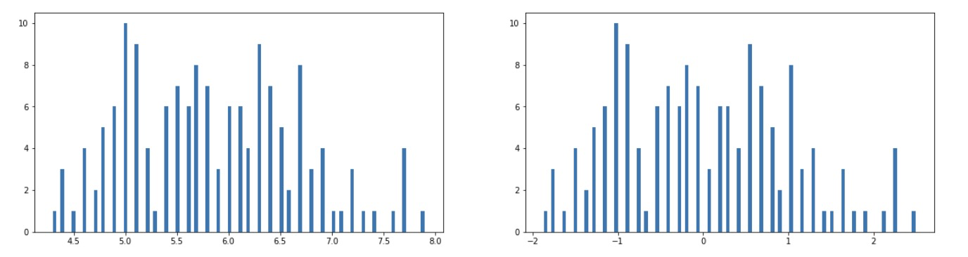
3.2} standardize the data and select a dimension to visualize the effect after processing

'''
Task 2:
Standardize the data and select a dimension to visualize the effect after processing 
'''
# 4. Data standardization preprocessing, variance mean=0, standard deviation std=1
from sklearn.preprocessing import StandardScaler
X_norm = StandardScaler().fit_transform(X)
print(X_norm)

# 5. Calculate variance mean and standard deviation sigma
#calcualte the mean and sigma
x1_mean = X.loc[:,'sepal length'].mean()
x1_norm_mean = X_norm[:,0].mean()
x1_sigma = X.loc[:,'sepal length'].std()
x1_norm_sigma = X_norm[:,0].std()
print(x1_mean,x1_sigma,x1_norm_mean,x1_norm_sigma)

# 6. Visualization: histogram comparison between original data and standardized data
%matplotlib inline
from matplotlib import pyplot as plt
fig1 = plt.figure(figsize=(20,5))

plt.subplot(121)
plt.hist(X.loc[:,'sepal length'],bins=100)

plt.subplot(122)
plt.hist(X_norm[:,0],bins=100)

plt.show()

fig1:

3.3 conduct PCA with the original data and other dimensions to view the variance proportion of each principal component

'''
Task 3:
Compare with the original data and other dimensions PCA，View the variance proportion of each principal component 
'''
# 7. PCA analysis: data obtained after dimensionality reduction by model training
#pca analysis
from sklearn.decomposition import PCA
pca = PCA(n_components=4)
X_pca = pca.fit_transform(X_norm)

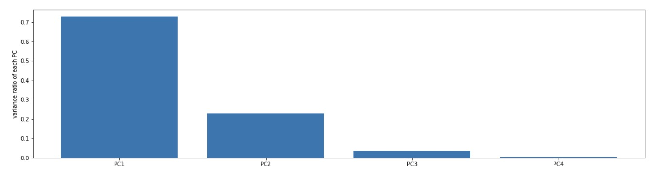
# 8. Calculate the variance ratio of principal components
#calculate the variance ratio of each principle components
var_ratio = pca.explained_variance_ratio_
print(var_ratio)
# Results: only the first two principal components were retained, that is, the dimension was reduced from 4 to 2

# 9. Visual variance ratio
fig2 = plt.figure(figsize=(20,5))
plt.bar([1,2,3,4],var_ratio)
plt.xticks([1,2,3,4],['PC1','PC2','PC3','PC4'])
plt.ylabel('variance ratio of each PC')
plt.show()

# 10. Just keep the first two principal components, i.e. 4D - > 2D, and the variance ratio of the latter two is small
pca = PCA(n_components=2)
X_pca = pca.fit_transform(X_norm)
X_pca.shape
type(X_pca)

fig2:

3.4 retain appropriate principal components and visualize the data after dimensionality reduction

'''
Task 4:
Retain the appropriate principal components and visualize the dimensionally reduced data
'''
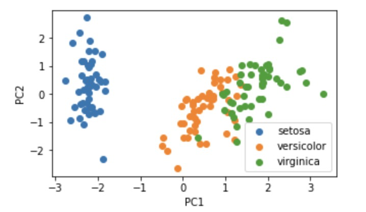
# 11. Visualize 2D data
#visualize the PCA result
fig3 = plt.figure(figsize=(5,3))
setosa=plt.scatter(X_pca[:,0][y==0],X_pca[:,1][y==0])
versicolor=plt.scatter(X_pca[:,0][y==1],X_pca[:,1][y==1])
virginica=plt.scatter(X_pca[:,0][y==2],X_pca[:,1][y==2])
plt.legend((setosa,versicolor,virginica),('setosa','versicolor','virginica'))
plt.xlabel('PC1')
plt.ylabel('PC2')
plt.show()

# Save drawing
fig3.savefig('1.png')