pandas practical method
catalogue
0. View Pandas version information
1.1 CSV file read data - read_csv()
1.2CSV file write data - to_csv()
1.3 reading data from excel file - read_excel()
1.4 EXCEL file write data - to_excel()
2. View the data of the first 5 rows or the last 5 rows
2.1 viewing the first 5 rows of data - head()
2.2 view the last 3 lines of data - tail()
3. View data dimensions, feature names, and feature types
3.1 view data dimension - shape
3.2 view data feature name - columns
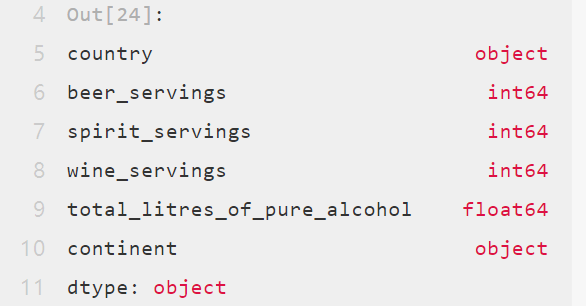
3.3 view some general information of DataFrame - info()
3.4 viewing basic statistical values of DataFrame - describe()
3.4. 1. View the basic statistical values of numerical characteristics in DataFrame
3.4. 2 view statistics of non numerical characteristics
3.5 viewing data types - dtypes
3.8 rename column name - rename()
4. Change the type of column - astype()
5. View feature distribution such as category and Boolean value - value_counts()
6.1 sorting according to the value of a single column
6.2 sorting by multi column values
7.1 get a separate column according to the column name - DataFrame['Name ']
7.2 indexing with Boolean values
7.5 first and last rows of dataframe
7.6 copy of dataframe - copy()
7.8 find the smallest column in the DataFrame table - idxmin()/idxmax()
7.9} DataFrame grouping, and get the sum of the maximum three numbers in each group
7.10 check the number of cities - unique()
7.11 delete duplicate data drop_duplicates()
7.13 calculation of correlation coefficient - corr()
7.14 calculate YoY -pct_change()
7.15 add prefix or suffix - add to column names_ Prefix() or add_suffix()
7.16 reset index reset_index()
7.17 select column by data type - select_dtypes()
7.18 building a dataframe glob module from multiple files
8. Apply functions to cells, columns, rows - apply()
9.1 replace the value in a column - map()
9.2 replace the value in a column - replace()
11.1. 1. Creation of pivot table
11.1. 2. Default value processing of pivot table
11.2. 1. Distribution according to occurrence frequency
11.2. 2 distribution according to occurrence proportion
12. Increase or decrease rows and columns of DataFrame
12.2 deleting columns and rows - drop()
13. DataFrame missing value operation
13.1 judge whether the DataFrame element is empty - isnull()
13.2 fill in missing values - fillna(value)
13.3 delete rows with missing values - dropna(how="any")
13.4 missing value fitting - interpolate()
13.6 remove extra characters in column data - extract()
14.1 convert string to lowercase letter - lower()
14.2 converting strings to uppercase letters
14.3 initial capitalization ()
15. Multi table join of DataFrame
15.1 merge by specified column - merge(left, right, on="key")
15.2 splicing multiple dataframe concat () using lists
16.1 establish a Series with time as index and random number as value
16.2 sum of corresponding values of each Wednesday in statistics s#
16.3} average value of monthly value in statistics s
16.4 converting time in Series (seconds to minutes)
16.6 conversion of different time representations
17.1 creating a DataFrame based on multiple indexes
17.2 multi index setting column name
17.3 DataFrame row column name conversion - stack()
17.4 DataFrame index conversion - unstack()
18.2 scatter diagram of dataframe
18.3 column diagram of dataframe
18.4 setting the size of the drawing
18.5 Chinese garbled codes and symbols are not displayed
19. Reduce DataFrame space size
0. View Pandas version information
import pandas as pd print(pd.__version__)
1. DataFrame file operation
1.1 CSV file read data - read_csv()
pd.read_csv(filepath_or_buffer,header,parse_dates,index_col)
import numpy as np
import pandas as pd
import warnings
warnings.filterwarnings('ignore')
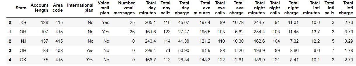
df = pd.read_csv( 'https://labfile.oss.aliyuncs.com/courses/1283/telecom_churn.csv')
df1.2CSV file write data - to_csv()
df3.to_csv('animal.csv')
print("Write successful.")
1.3 reading data from excel file - read_excel()
pd.read_excel('animal.xlsx', 'Sheet1', index_col=None, na_values=['NA'])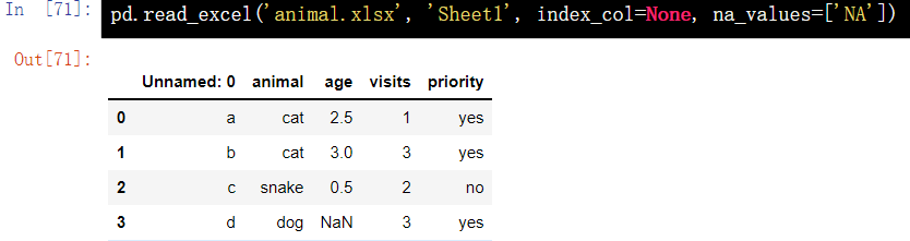
1.4 EXCEL file write data - to_excel()
df3.to_excel('animal.xlsx', sheet_name='Sheet1')
print("Write successful.")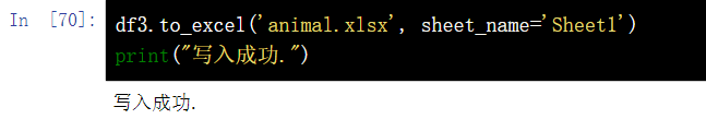
2. View the data of the first 5 rows or the last 5 rows
2.1 viewing the first 5 rows of data - head()
df.head()
2.2 view the last 3 lines of data - tail()
df.tail(3)
3. View data dimensions, feature names, and feature types
3.1 view data dimension - shape
# View data dimensions
df.shape

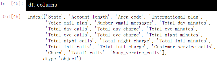
3.2 view data feature name - columns
# View data feature name
df.columns
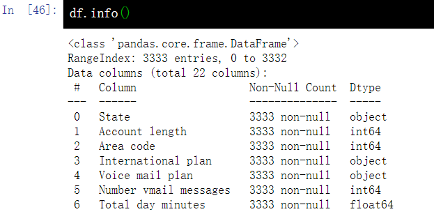
3.3 view some general information of DataFrame - info()
# View some general information about the DataFrame
df.info()
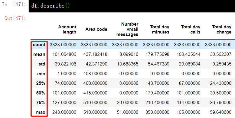
3.4 viewing basic statistical values of DataFrame - describe()
3.4. 1. View the basic statistical values of numerical characteristics in DataFrame
# View the basic statistical values of numerical features in the DataFrame, such as values without missing values, mean values, standard deviations, etc
df.describe()
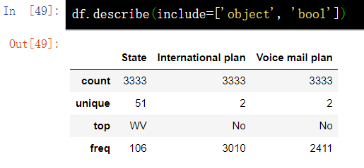
3.4. 2 view statistics of non numerical characteristics
#You can view statistics for non numeric characteristics by explicitly specifying the type of data to include with the include parameter.
df.describe(include=['object', 'bool'])
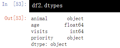
3.5 viewing data types - dtypes
df2.dtypes
3.6 view index
df.index
3.7 view values
df.values
3.8 rename column name - rename()
df.rename(columns={"category":"category-size"})4. Change the type of column - astype()
df['Churn'] = df['Churn'].astype('int64')5. View feature distribution such as category and Boolean value - value_counts()
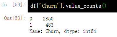
5.1 by occurrence frequency
df['Churn'].value_counts()
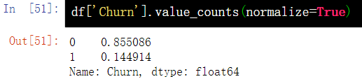
5.2 proportion of occurrence
df['Churn'].value_counts(normalize=True)
6. Sort sort_values()
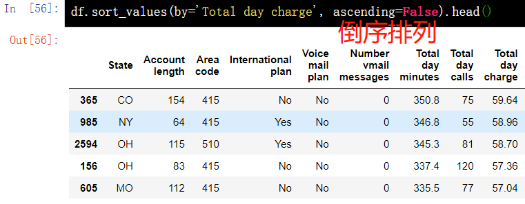
6.1 sorting according to the value of a single column
df.sort_values(by='Total day charge', ascending=False).head()
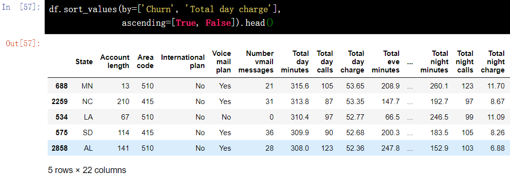
 6.2 sorting by multi column values
df.sort_values(by=['Churn', 'Total day charge'], ascending=[True, False]).head()
7. Get data
7.1 get a separate column according to the column name - DataFrame['Name ']
df['Churn'].mean()
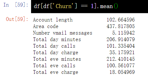
7.2 indexing with Boolean values
df[df['Churn'] == 1].mean()

df[(df['Churn'] == 0) & (df['International plan'] == 'No') ]['Total intl minutes'].max()
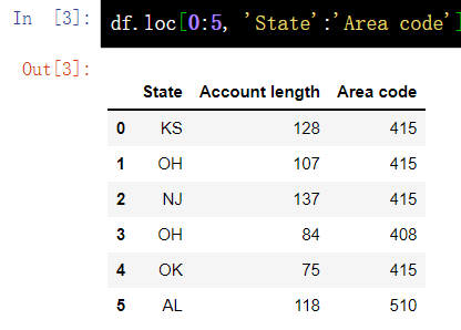
7.3 by name index - loc
df.loc[0:5, 'State':'Area code']
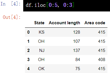
7.4 by numerical index -iloc
df.iloc[0:5, 0:3]
7.5 first and last rows of dataframe
df[:1]
df[-1:]
7.6 copy of dataframe - copy()
df = df2.copy()
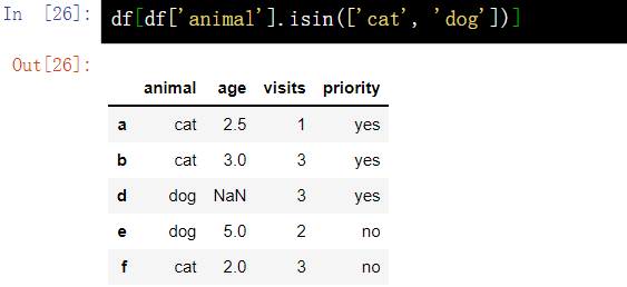
7.7 query by keyword - isin()
df[df['animal'].isin(['cat', 'dog'])]
7.8 find the smallest column in the DataFrame table - idxmin()/idxmax()
df = pd.DataFrame(np.random.random(size=(5, 5)), columns=list('abcde'))
print(df)
df.sum().idxmin() # idxmax(), idxmin() returns the index value of the maximum and minimum value for the Series function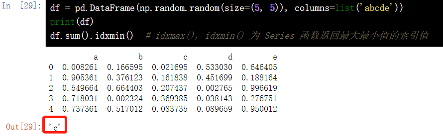 7.9} DataFrame grouping, and get the sum of the maximum three numbers in each group
df = pd.DataFrame({'A': list('aaabbcaabcccbbc'), 'B': [12, 345, 3, 1, 45, 14, 4, 52, 54, 23, 235, 21, 57, 3, 87]})
print(df)
df.groupby('A')['B'].nlargest(3).sum(level=0)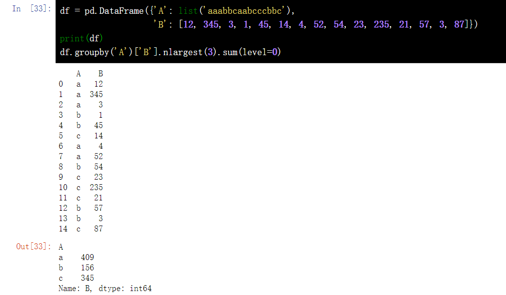
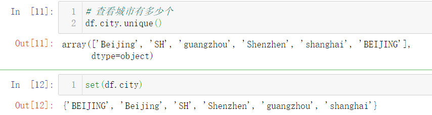
7.10 check the number of cities - unique()
df.city.unique()
set(df.city)
 7.11 delete duplicate data drop_duplicates()
 # Delete duplicate data DF city. str.lower(). drop_ duplicates()
df.city.str.lower().drop_duplicates(keep="last")
df.city.str.lower().replace("sh","shanghai").drop_duplicates()
7.12 data filtering query()
# Filter using the query function
df.query('city==["beijing","shanghai"]')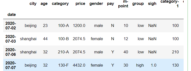
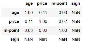
7.13 calculation of correlation coefficient - corr()
# Correlation coefficient between m-point and price
df_inner["price"].corr(df_inner["m-point"])

# Correlation coefficient of whole data and numerical variables
df_inner.corr().round(2)
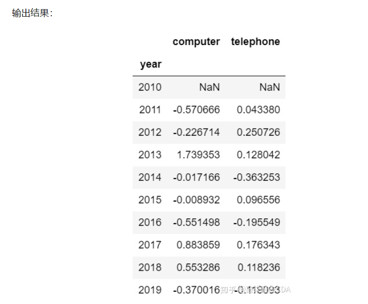
7.14 calculate YoY -pct_change()
df1.pct_change() #Calculates the percentage change between the current element and the previous element
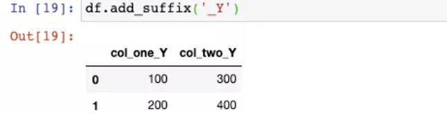
7.15 add prefix or suffix - add to column names_ Prefix() or add_suffix()
df.add_prefix("X_")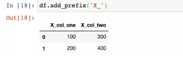
df.add_suffix()
7.16 reset index reset_index()
df.reset_index(drop=True)
7.17 select column by data type - select_dtypes()
df.select_dtypes(include="number").head()
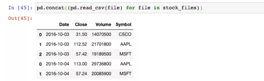
7.18 building a dataframe glob module from multiple files
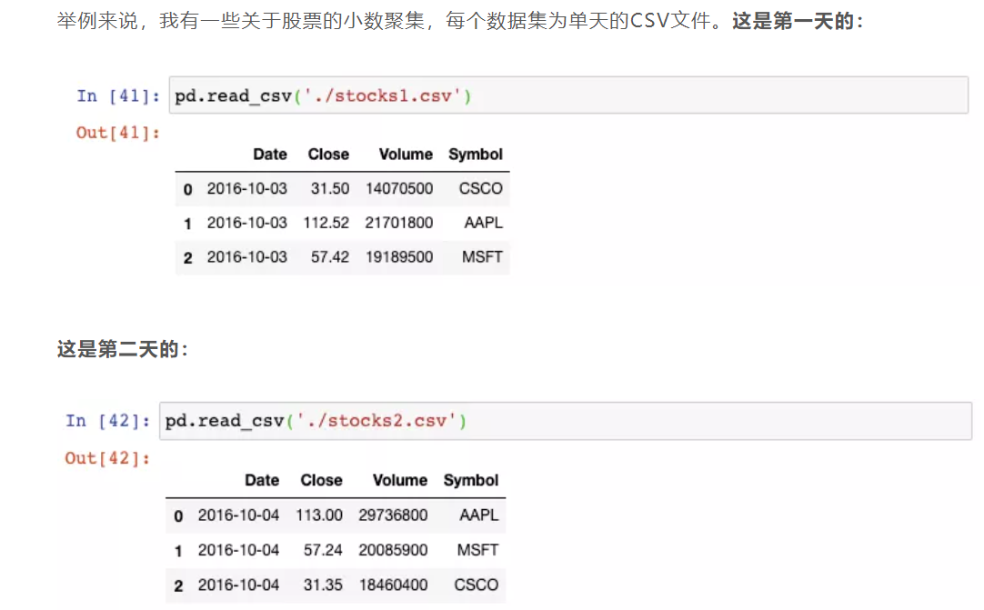
from glob import glob
stock_files = sorted(glob("stock*.csv))
stock_files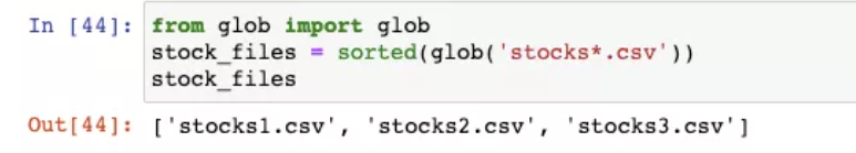
pd.concat((pd.read_csv(file) for file in stock_files))
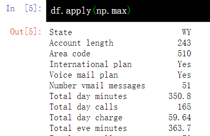
8. Apply functions to cells, columns, rows - apply()
8.1 apply to columns
df.apply(np.max)
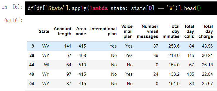
8.2 apply to each line
The apply() method can also apply the function to each line by specifying axis=1. In this case, it is convenient to use the lambda function. For example, the following function selects all States starting with W.
df[df['State'].apply(lambda state: state[0] == 'W')].head()
9. Replace value
9.1 replace the value in a column - map()
d = {'No': False, 'Yes': True}
df['International plan'] = df['International plan'].map(d)
df.head()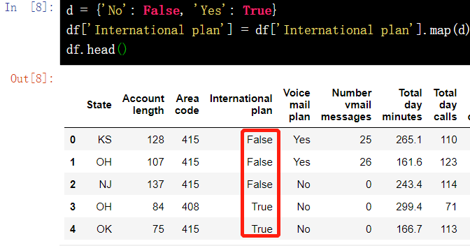
9.2 replace the value in a column - replace()
df = df.replace({'Voice mail plan': d})
df.head()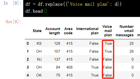
10. Group by ()
The general form of packet data in pandas is:
df.groupby(by=grouping_columns)[columns_to_show].function()
- The groupby() method is based on grouping_columns.
- Next, select the columns_to_show of interest. If this item is not included, all non group by columns (i.e. all columns except grouping_columns) will be selected.
- Finally, apply one or more function s.
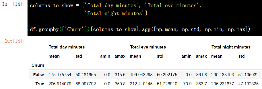
columns_to_show = ['Total day minutes', 'Total eve minutes', 'Total night minutes']
df.groupby(['Churn'])[columns_to_show].describe(percentiles=[])

It is similar to the above example, except that this time some functions are passed to {agg(), and the grouped data is aggregated through the} agg() method.
columns_to_show = ['Total day minutes', 'Total eve minutes', 'Total night minutes']
df.groupby(['Churn'])[columns_to_show].agg([np.mean, np.std, np.min, np.max])
11. Summary / PivotTable
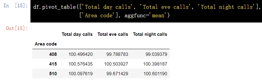
11.1 pivot table_ table()
The pivot table in Pandas is defined as follows:
Pivot table is a common data summary tool in spreadsheet programs and other data exploration software. It aggregates data according to one or more keys and distributes data into rectangular areas according to grouping on rows and columns.
Via {pivot_ The table () method can create a pivot table with the following parameters:
- values represents the variable list of statistics to be calculated
- index represents the variable list of grouped data
- aggfunc indicates which statistics need to be calculated, such as sum, mean, maximum, minimum, etc.
11.1. 1. Creation of pivot table
df.pivot_table(['Total day calls', 'Total eve calls', 'Total night calls'], ['Area code'], aggfunc='mean')
pd.pivot_table(df, values=['D'], index=['A', 'B'], aggfunc=[np.sum, len])
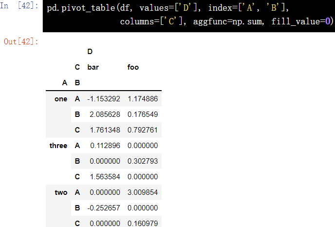
11.1. 2. Default value processing of pivot table
pd.pivot_table(df, values=['D'], index=['A', 'B'], columns=['C'], aggfunc=np.sum, fill_value=0)
11.2 crosstab()
Cross Tabulation is a special pivot table used to calculate the grouping frequency. In Pandas, the cross table is generally constructed using the {crosstab() method.
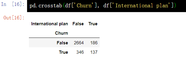
11.2. 1. Distribution according to occurrence frequency
pd.crosstab(df['Churn'], df['International plan'])
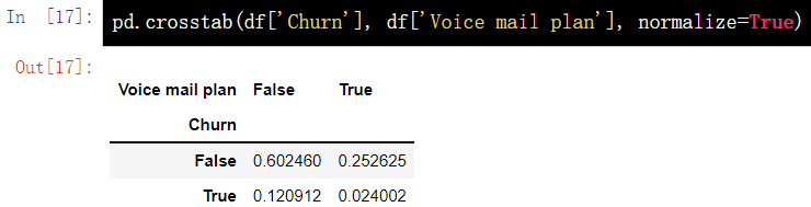
11.2. 2 distribution according to occurrence proportion
pd.crosstab(df['Churn'], df['Voice mail plan'], normalize=True)
12. Increase or decrease rows and columns of DataFrame
12.1 method of adding columns
12.1.1 insert()
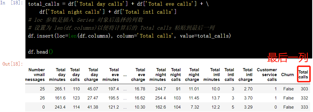
total_calls = df['Total day calls'] + df['Total eve calls'] + \ df['Total night calls'] + df['Total intl calls']
# The loc parameter is the number of columns selected after the Series object is inserted
# Set to len(df.columns) to paste the calculated Total calls to the last column
df.insert(loc=len(df.columns), column='Total calls', value=total_calls)
df.head()
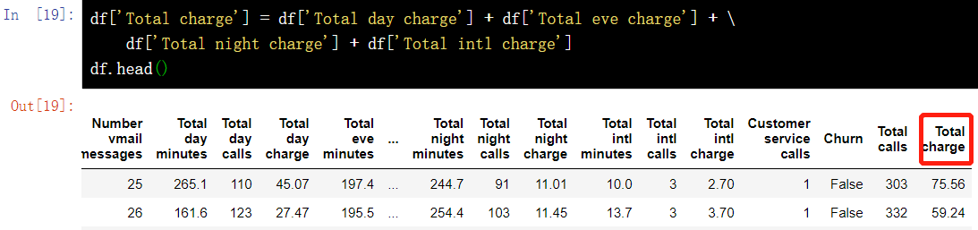
12.1. 2 add directly
df['Total charge'] = df['Total day charge'] + df['Total eve charge'] + \ df['Total night charge'] + df['Total intl charge']
df.head()
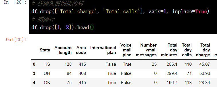
12.2 deleting columns and rows - drop()
# Remove previously created columns
df.drop(['Total charge', 'Total calls'], axis=1, inplace=True)
# Delete row
df.drop([1, 2]).head()
13. DataFrame missing value operation
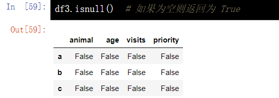
13.1 judge whether the DataFrame element is empty - isnull()
df.isnull()
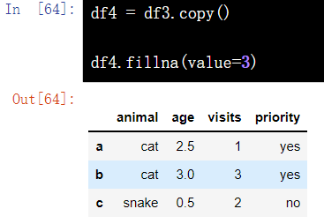
13.2 fill in missing values - fillna(value)
df4 = df3.copy() df4.fillna(value=3)
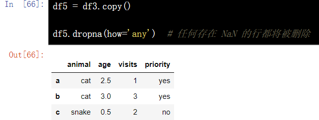
13.3 delete rows with missing values - dropna(how="any")
df5 = df3.copy() df5.dropna(how='any') # Any rows with NaN will be deleted
13.4 missing value fitting - interpolate()
df = pd.DataFrame({'From_To': ['LoNDon_paris', 'MAdrid_miLAN', 'londON_StockhOlm', 'Budapest_PaRis', 'Brussels_londOn'], 'FlightNumber': [10045, np.nan, 10065, np.nan, 10085], 'RecentDelays': [[23, 47], [], [24, 43, 87], [13], [67, 32]], 'Airline': ['KLM(!)', '<Air France> (12)', '(British Airways. )', '12. Air France', '"Swiss Air"']})
df['FlightNumber'] = df['FlightNumber'].interpolate().astype(int)
df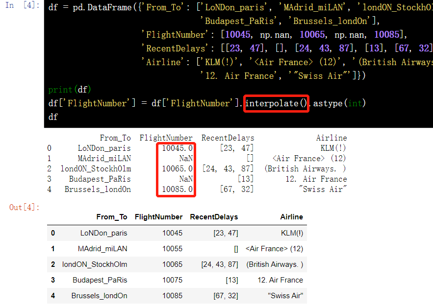
13.5 data column splitting
temp = df.From_To.str.split('_', expand=True)
temp.columns = ['From', 'To']
temp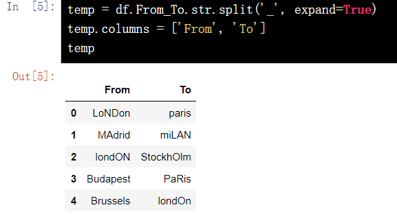
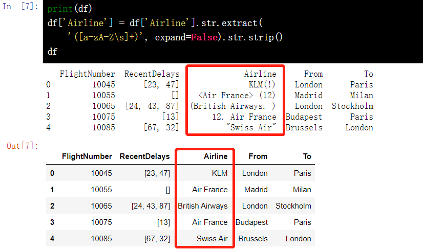
13.6 remove extra characters in column data - extract()
df['Airline'] = df['Airline'].str.extract( '([a-zA-Z\s]+)', expand=False).str.strip()
df
13.7 format specification
delays = df['RecentDelays'].apply(pd.Series)
delays.columns = ['delay_{}'.format(n) for n in range(1, len(delays.columns)+1)]
df = df.drop('RecentDelays', axis=1).join(delays)
df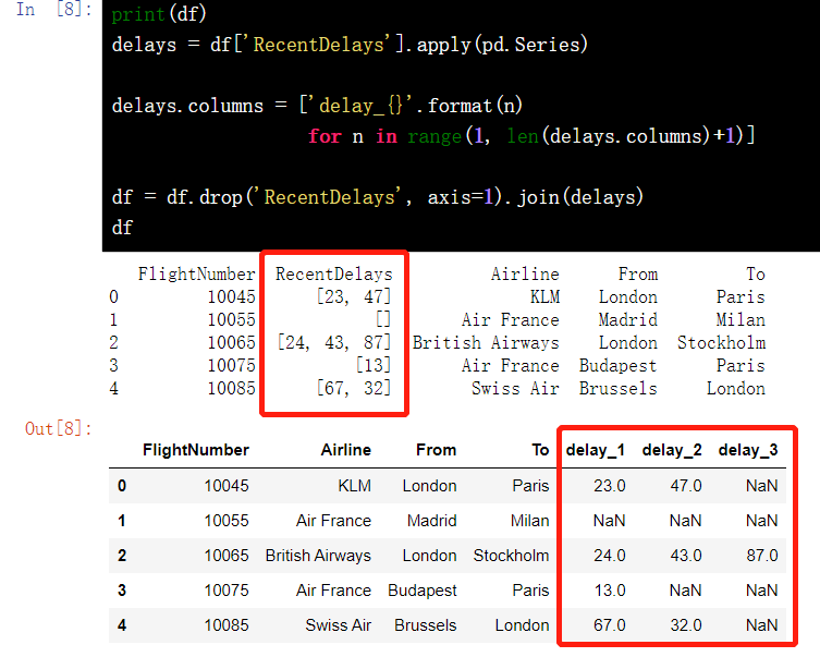
14. String operation
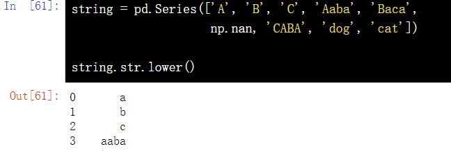
14.1 convert string to lowercase letter - lower()
string = pd.Series(['A', 'B', 'C', 'Aaba', 'Baca', np.nan, 'CABA', 'dog', 'cat'])
string.str.lower()
14.2 converting strings to uppercase letters
string.str.upper()
14.3 initial capitalization ()
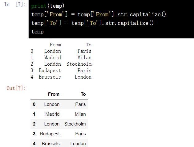
print(temp) temp['From'] = temp['From'].str.capitalize()
temp['To'] = temp['To'].str.capitalize()
temp
15. Multi table join of DataFrame
15.1 merge by specified column - merge(left, right, on="key")
The number of rows in the result set does not increase, and the number of columns is the number of columns of the two metadata and minus the number of join keys.
DataFrame.merge(left, right, how='inner', on=None, left_on=None, right_on =None, left_index=False, right_index=False, sort=False, suffixes=('_x', '_y'), copy=True, indicator=False, validate =None)[source]left = pd.DataFrame({'key': ['foo1', 'foo2'], 'one': [1, 2]})
right = pd.DataFrame({'key': ['foo2', 'foo3'], 'two': [4, 5]})
# Align the connection according to the key column. Only foo2 is the same, so it finally becomes a row
pd.merge(left, right, on='key')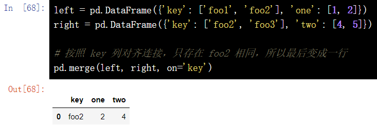
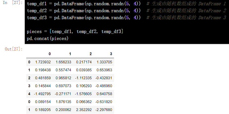
15.2 splicing multiple dataframe concat () using lists
Vertical stack of CONCAT. Vertical stacking is axis=0. In this case, there is a special parameter called 'ignore'_ Index = ', False by default. If it is set to True, the resulting consolidated table is re indexed. Otherwise, the row index is still the value in the original two tables
pandas.concat(objs, axis=0, join='outer', join_axes=None, ignore_index= False, keys=None, levels=None, names=None, verify_integrity= False, sort=None, copy=True)
temp_df1 = pd.DataFrame(np.random.randn(5, 4)) # Generate DataFrame 1 composed of random numbers
temp_df2 = pd.DataFrame(np.random.randn(5, 4)) # Generate DataFrame 2 composed of random numbers
temp_df3 = pd.DataFrame(np.random.randn(5, 4)) # Generate DataFrame 3 composed of random numbers
pieces = [temp_df1, temp_df2, temp_df3]
pd.concat(pieces)
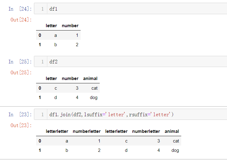
15.3 splicing column join()
JOIN spliced columns are mainly used for merging based on row indexes.
As long as the column names of the two tables are different, they can be used directly without adding any parameters; If two tables have duplicate column names, lsuffix and rsuffix parameters need to be specified; The meaning of the parameter is basically the same as that of the merge method, except that the join method defaults to the left outer connection how=left
DataFrame.join(other, on=None, how='left', lsuffix='', rsuffix='', sort= False)
df1.join(df2,lsuffix="letter",rsuffix="lerrer)
16. Time series processing
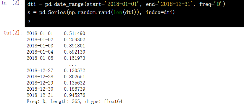
16.1 establish a Series with time as index and random number as value
dti = pd.date_range(start='2018-01-01', end='2018-12-31', freq='D')
s = pd.Series(np.random.rand(len(dti)), index=dti)
s
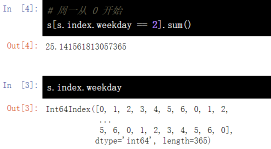
16.2 sum of corresponding values of each Wednesday in statistics s#
# Monday from 0
s[s.index.weekday == 2].sum()
16.3} average value of monthly value in statistics s
s.resample('M').mean()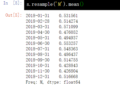
16.4 converting time in Series (seconds to minutes)
s = pd.date_range('today', periods=100, freq='S')
ts = pd.Series(np.random.randint(0, 500, len(s)), index=s)
ts.resample('Min').sum()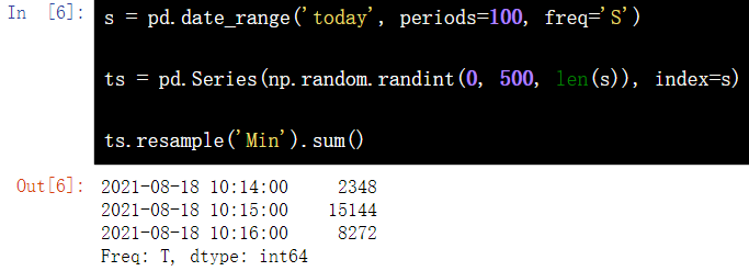
16.5 UTC world time standard
s = pd.date_range('today', periods=1, freq='D') # Get current time
ts = pd.Series(np.random.randn(len(s)), s) # Random value
ts_utc = ts.tz_localize('UTC') # Convert to UTC time
ts_utc
Convert to Shanghai time zone
ts_utc.tz_convert('Asia/Shanghai')16.6 conversion of different time representations
rng = pd.date_range('1/1/2018', periods=5, freq='M')
ts = pd.Series(np.random.randn(len(rng)), index=rng)
print(ts)
ps = ts.to_period()
print(ps)
ps.to_timestamp()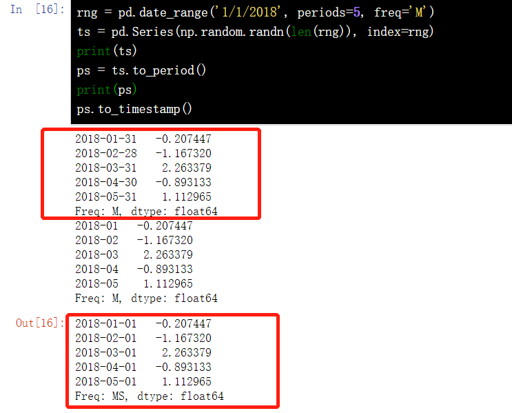
17. DataFrame multiple index
17.1 creating a DataFrame based on multiple indexes
frame = pd.DataFrame(np.arange(12).reshape(6, 2), index=[list('AAABBB'), list('123123')], columns=['hello', 'shiyanlou'])
frame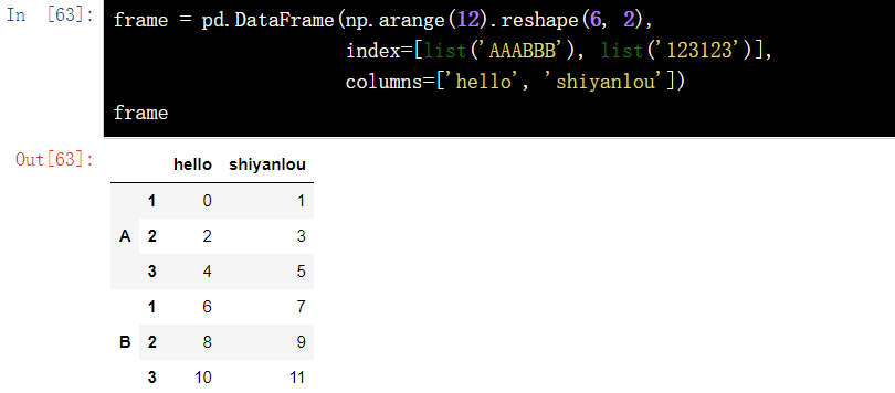
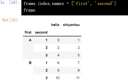
17.2 multi index setting column name
frame.index.names = ['first', 'second']
frame
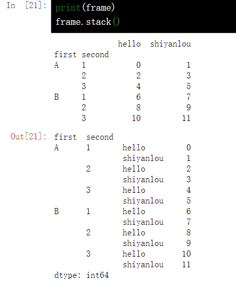
17.3 DataFrame row column name conversion - stack()
stack() turns the original column index (A, B) into the innermost row index (ABAB)
print(frame)
frame.stack()
17.4 DataFrame index conversion - unstack()
The unstack() method is very similar to the pivot() method. The main difference is that the unstack() method is for indexes or labels, that is, the column index is transformed into the innermost row index; The pivot() method is for the value of the column, that is, specify the value of a column as the row index, specify the value of a column as the column index, and then specify which columns as the corresponding values of the index
print(frame)
frame.unstack()

18. Pandas drawing operation
18.1 DataFrame line chart
f = pd.DataFrame({"xs": [1, 5, 2, 8, 1], "ys": [4, 2, 1, 9, 6]})
df = df.cumsum()
df.plot()
18.2 scatter diagram of dataframe
df = pd.DataFrame({"xs": [1, 5, 2, 8, 1], "ys": [4, 2, 1, 9, 6]})
df = df.cumsum()
df.plot.scatter("xs", "ys", color='red', marker="*")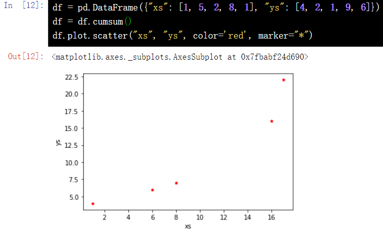
18.3 column diagram of dataframe
df = pd.DataFrame({"revenue": [57, 68, 63, 71, 72, 90, 80, 62, 59, 51, 47, 52], "advertising": [2.1, 1.9, 2.7, 3.0, 3.6, 3.2, 2.7, 2.4, 1.8, 1.6, 1.3, 1.9], "month": range(12) })
ax = df.plot.bar("month", "revenue", color="yellow")
df.plot("month", "advertising", secondary_y=True, ax=ax)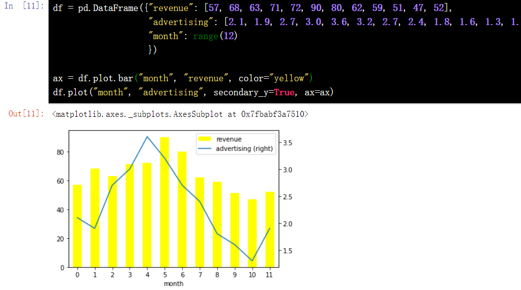
18.4 setting the size of the drawing
Method 1:
%pylab inline figsize(16, 6)
Method 2:
import matplotlib.pyplot as plt
plt.style.use({'figure.figsize':(12, 6)})
18.5 Chinese garbled codes and symbols are not displayed
plt.rcParams['font.sans-serif'] = ['SimHei']
plt.rcParams['axes.unicode_minus'] =False
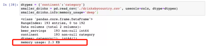
19. Reduce DataFrame space size
19.1 viewing space usage
drinks.info(memory_usage="deep")

19.2 reduce space size
1) Read only the columns actually needed
cols= ["beer_servings","continent"]
small_drinks = pd.read_csv("./drinksbycountry.csv",usecols=cols)
small_drinks.info(memory_usage="deep")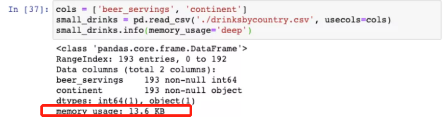
2) Convert all object columns that are actually category variables to category variables
dtypes={"continent":"category"}
smaller_drinks = pd.read_csv("./drinksbycountry.csv",usecols=cols,dtype=dtypes)
smaller_drinks.info(memory_usage="deep")