Note: the tutorial content is from https://nbviewer.jupyter.org/github/twiecki/financial-analysis-python-tutorial/tree/master/ This is not a complete system pandas tutorial. The test demo of this foreign tutorial is old, and the new version of pandas may not be compatible with the source program. This tutorial is a correction based on the original tutorial Test with Spyder IDE

# -*- coding: utf-8 -*-
"""
Created on Sun Mar 29 17:58:13 2020

@author: CHERN
"""

import datetime
import pandas as pd
from pandas import Series, DataFrame
print(pd.__version__)

import matplotlib.pyplot as plt
import matplotlib as mpl
mpl.rc('figure', figsize=(8, 7))
print(mpl.__version__)

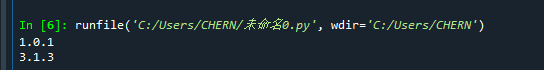
The test program uses pandas version 1.0.1 and Matplotlib version 3.1.3

1. Create and load data

1.1 generated according to python built-in list/dict

# -*- coding: utf-8 -*-
"""
Created on Sun Mar 29 17:58:13 2020

@author: CHERN
"""

import datetime
import pandas as pd
from pandas import Series, DataFrame
# print(pd.__version__)

import matplotlib.pyplot as plt
import matplotlib as mpl
mpl.rc('figure', figsize=(8, 7))
# print(mpl.__version__)

# Constructing one-dimensional sequence through python
labels = ['a', 'b', 'c', 'd', 'e']
s = Series([1, 2, 3, 4, 5], index=labels)
print(s)
print(r"'b' in s?")
print('b' in s)
print(s['b'])

print("Series.to_dict() can convert Series to dict")
mapping = s.to_dict()
print(mapping)

print("Series(dict) can convert dict to Series")
print(Series(mapping))

[the external chain image transfer fails. The source station may have an anti-theft chain mechanism. It is recommended to save the image and upload it directly (img-eKV3iS94-1586606244035)(assets/2020-03-29-18-12-01.png)]

Usage Summary

1. The constructor of Series object can pass dict dictionary type variable or use list in python
2. Series. to_ The dict () method can convert series objects into python built-in dict objects
3. Through 'b' in s, you can judge whether the key 'b' exists in the index of the Series object, and the return value is True/False
4. s['b '] can obtain data in Series

1.2 get from the network

# -*- coding: utf-8 -*-
"""
Created on Sun Mar 29 17:58:13 2020

@author: CHERN
"""

import datetime
import pandas as pd
from pandas import Series, DataFrame
# print(pd.__version__)

import numpy as np
from pandas_datareader import data, wb # PIP install pandas needs to be installed_ datareader

import matplotlib.pyplot as plt
import matplotlib

import matplotlib as mpl
mpl.rc('figure', figsize=(8, 7))
# print(mpl.__version__)


# Define the time period for obtaining data
start = datetime.datetime(2010, 1, 1)
end = datetime.datetime(2016,5,20)
sh = data.DataReader("000001.SS", 'yahoo', start, end)
print(sh.head(3)) # First three lines of output data

# Pandas will be obtained from Yahoo Save dataframe data to csv file
sh.to_csv('sh.csv')

be careful:

1. Version updated, previous PD io. data. get_ data_ Yahoo () method has been deprecated. DataReader method is currently used for experimental operation
2. Domestic data access may be slow, so VPN needs to be enabled For the sake of simplicity (the code is reused directly without other files), the following case will be carried out according to the data obtained from the Internet

Usage Summary:

1. from pandas_ After datareader imports data, data The datareader () method can obtain financial data (stock history data) from the network
2. DataFrame object can be used if there are too many rows The head() method outputs its first five lines head(n) output the first n lines

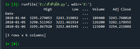
Note: here, Date is the index of the object sh

1.3 read data from file (. CSV /. Xlsx, etc.)

# -*- coding: utf-8 -*-
"""
Created on Sun Mar 29 17:58:13 2020

@author: CHERN
"""

import datetime
import pandas as pd
from pandas import Series, DataFrame
# print(pd.__version__)

import numpy as np
from pandas_datareader import data, wb # PIP install pandas needs to be installed_ datareader

import matplotlib.pyplot as plt
import matplotlib

import matplotlib as mpl
mpl.rc('figure', figsize=(8, 7))
# print(mpl.__version__)


# Define the time period for obtaining data
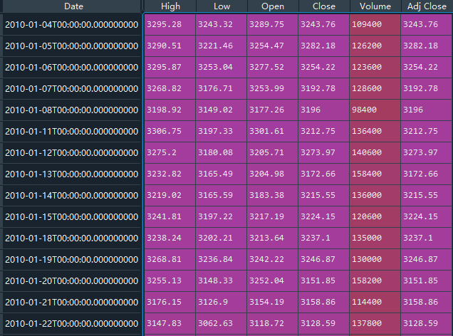
df = pd.read_csv('sh.csv', index_col='Date', parse_dates=True)
print(df)

2. Series and DataFrame: (basic operation)

2.1 index slice create new column

# -*- coding: utf-8 -*-
"""
Created on Sun Mar 29 17:58:13 2020

@author: CHERN
"""

import datetime
import pandas as pd
from pandas import Series, DataFrame
# print(pd.__version__)

import numpy as np
from pandas_datareader import data, wb # PIP install pandas needs to be installed_ datareader

import matplotlib.pyplot as plt
import matplotlib

import matplotlib as mpl
mpl.rc('figure', figsize=(8, 7))
# print(mpl.__version__)


# Define the time period for obtaining data
df = pd.read_csv('sh.csv', index_col='Date', parse_dates=True)
# print(df)

# type(ts) = pandas.core.series.Series
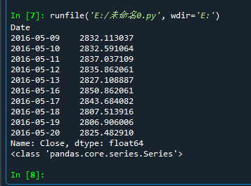
ts = df['Close'][-10:]
print(ts)
print(type(ts))

Continue in IPython:

date = ts.index[5]
date

Output:

Timestamp('2016-05-16 00:00:00')

Input:

ts[date]

Output:

2850.862060546875

Input:

ts[5]

Output:

2850.862060546875

Input:

df[['Open', 'Close']].head()

Output:

                   Open        Close
Date                                
2010-01-04  3289.750000  3243.760010
2010-01-05  3254.468018  3282.178955
2010-01-06  3277.517090  3254.215088
2010-01-07  3253.990967  3192.775879
2010-01-08  3177.259033  3195.997070

Input:

df['diff'] = df.Open - df.Close
df.head()

Output:

                   High          Low  ...    Adj Close       diff
Date                                  ...                        
2010-01-04  3295.279053  3243.319092  ...  3243.760010  45.989990
2010-01-05  3290.511963  3221.461914  ...  3282.178955 -27.710938
2010-01-06  3295.867920  3253.043945  ...  3254.215088  23.302002
2010-01-07  3268.819092  3176.707031  ...  3192.775879  61.215088
2010-01-08  3198.919922  3149.017090  ...  3195.997070 -18.738037

[5 rows x 7 columns]

Input:

del df['diff']
df.head()

Output:

                   High          Low  ...  Volume    Adj Close
Date                                  ...                     
2010-01-04  3295.279053  3243.319092  ...  109400  3243.760010
2010-01-05  3290.511963  3221.461914  ...  126200  3282.178955
2010-01-06  3295.867920  3253.043945  ...  123600  3254.215088
2010-01-07  3268.819092  3176.707031  ...  128600  3192.775879
2010-01-08  3198.919922  3149.017090  ...   98400  3195.997070

[5 rows x 6 columns]

Usage Summary:

1. The instruction del df['diff'] can delete the 'diff' column in the data df

3. Conventional financial calculation

3.1 moving average

close_px = df['Adj Close']
mavg = pd.rolling_mean(close_px, 40)
mavg[-10:]

Output:

  File "<ipython-input-14-9dd3f0f7e3fa>", line 2, in <module>
    mavg = pd.rolling_mean(close_px, 40)

  File "C:\Python\lib\site-packages\pandas\__init__.py", line 262, in __getattr__
    raise AttributeError(f"module 'pandas' has no attribute '{name}'")

AttributeError: module 'pandas' has no attribute 'rolling_mean'

pandas version update, enabling rolling_ Method () mean

close_px = df['Adj Close']
mavg = close_px.rolling(40).mean()
mavg

Output:

Date
2010-01-04            NaN
2010-01-05            NaN
2010-01-06            NaN
2010-01-07            NaN
2010-01-08            NaN
    
2016-05-16    2970.439978
2016-05-17    2967.653333
2016-05-18    2962.371130
2016-05-19    2957.559705
2016-05-20    2952.947778
Name: Adj Close, Length: 1550, dtype: float64

3.2 revenue

Input:

rets = close_px / close_px.shift(1) - 1
# rets = close_px.pct_change()
rets.head()

Output:

Date
2010-01-04         NaN
2010-01-05    0.011844
2010-01-06   -0.008520
2010-01-07   -0.018880
2010-01-08    0.001009
Name: Adj Close, dtype: float64

4. Drawing basis

close_px.plot(label='AAPL')
mavg.plot(label='mavg')
plt.legend()

[the external chain picture transfer fails. The source station may have an anti-theft chain mechanism. It is recommended to save the picture and upload it directly (img-VS5moCnW-1586606244038)(assets/2020-03-29-20-40-41.png)]

Extend

# -*- coding: utf-8 -*-
"""
Created on Sun Mar 29 17:58:13 2020

@author: CHERN
"""

import datetime
import pandas as pd
from pandas import Series, DataFrame
# print(pd.__version__)

import numpy as np
from pandas_datareader import data, wb # PIP install pandas needs to be installed_ datareader

import matplotlib.pyplot as plt
import matplotlib

import matplotlib as mpl
mpl.rc('figure', figsize=(8, 7))
# print(mpl.__version__)


# Define the time period for obtaining data
start = datetime.datetime(2010, 1, 1)
end = datetime.datetime(2016,5,20)
sh = data.DataReader(['AAPL','GE','GOOG','IBM','KO', 'MSFT', 'PEP'],'yahoo', start, end)['Adj Close']
print(sh.head(3)) # First three lines of output data

Symbols          AAPL         GE        GOOG  ...         KO       MSFT        PEP
Date                                          ...                                 
2009-12-31  26.131752  10.526512  308.832428  ...  19.278732  23.925440  44.622261
2010-01-04  26.538483  10.749147  312.204773  ...  19.292267  24.294369  44.945187
2010-01-05  26.584366  10.804806  310.829926  ...  19.058893  24.302216  45.488274

[3 rows x 7 columns]

Input:

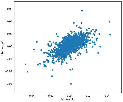
rets = df.pct_change()
plt.scatter(rets.PEP, rets.KO)
plt.xlabel('Returns PEP')
plt.ylabel('Returns KO')

pd.scatter_matrix(rets, diagonal='kde', figsize=(10, 10));

Output:

  File "C:\Python\lib\site-packages\pandas\__init__.py", line 262, in __getattr__
    raise AttributeError(f"module 'pandas' has no attribute '{name}'")

AttributeError: module 'pandas' has no attribute 'scatter_matrix'

Scatter of pandas_ Matrix usage has changed to pandas plotting. scatter_matrix

Re-enter:

pd.plotting.scatter_matrix(rets, diagonal='kde', figsize=(10, 10));

[the external chain image transfer fails. The source station may have an anti-theft chain mechanism. It is recommended to save the image and upload it directly (img-aAdqCmPm-1586606244040)(assets/2020-03-29-21-18-44.png)]

Knowledge summary:

1. Scatter chart is a tool used to judge the relationship between two variables. Generally, scatter chart uses two groups of data to form multiple coordinate points. By observing the distribution of coordinate points, it can judge whether there is a correlation relationship between variables and the strength of the correlation relationship. In addition, if there is no correlation, the scatter diagram can be used to summarize the distribution pattern of feature points, i.e. matrix diagram (quadrant diagram)
2. pd.scatter_matrix() and PD Scatter() is used to draw scatter matrix and scatter chart

Input:

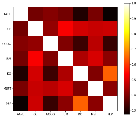
corr = rets.corr()
corr

Output:

Symbols      AAPL        GE      GOOG       IBM        KO      MSFT       PEP
Symbols                                                                      
AAPL     1.000000  0.387574  0.406971  0.387261  0.298461  0.393892  0.273217
GE       0.387574  1.000000  0.423675  0.532942  0.491217  0.478202  0.485198
GOOG     0.406971  0.423675  1.000000  0.402424  0.329096  0.463922  0.322701
IBM      0.387261  0.532942  0.402424  1.000000  0.449300  0.495341  0.412432
KO       0.298461  0.491217  0.329096  0.449300  1.000000  0.402174  0.643624
MSFT     0.393892  0.478202  0.463922  0.495341  0.402174  1.000000  0.414073
PEP      0.273217  0.485198  0.322701  0.412432  0.643624  0.414073  1.000000

Input:

plt.imshow(corr, cmap='hot', interpolation='none')
plt.colorbar()
plt.xticks(range(len(corr)), corr.columns)
plt.yticks(range(len(corr)), corr.columns);

Usage Summary:

1. pd. The corr () method is used to calculate the correlation between two sequences

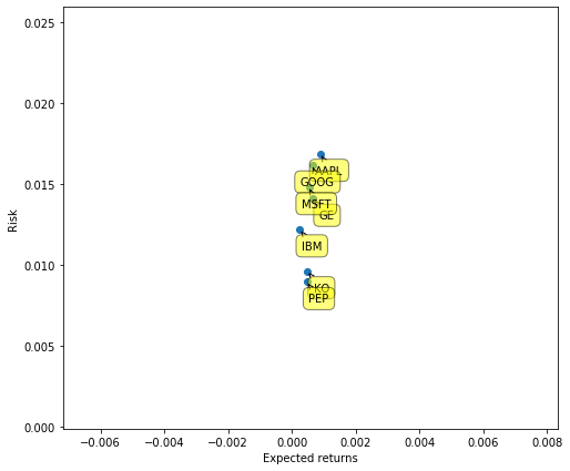
One thing we are often interested in is the relationship between the expected return (usually the mean of the rate of return) and the risk we take (the variance of the rate of return). There is often a trade-off between the two.
Here we use PLT Annotate labels the scatter chart.

plt.scatter(rets.mean(), rets.std())
plt.xlabel('Expected returns')
plt.ylabel('Risk')
for label, x, y in zip(rets.columns, rets.mean(), rets.std()):
    plt.annotate(
        label, 
        xy = (x, y), xytext = (20, -20),
        textcoords = 'offset points', ha = 'right', va = 'bottom',
        bbox = dict(boxstyle = 'round,pad=0.5', fc = 'yellow', alpha = 0.5),
        arrowprops = dict(arrowstyle = '->', connectionstyle = 'arc3,rad=0'))

5. Data alignment and Nan processing

Procedure:

# -*- coding: utf-8 -*-
"""
Created on Sun Mar 29 17:58:13 2020

@author: CHERN
"""

import datetime
import pandas as pd
from pandas import Series, DataFrame
# print(pd.__version__)

import numpy as np
from pandas_datareader import data, wb # PIP install pandas needs to be installed_ datareader

import matplotlib.pyplot as plt
import matplotlib

import matplotlib as mpl
mpl.rc('figure', figsize=(8, 7))
# print(mpl.__version__)


series_list = []
securities = ['AAPL', 'GOOG', 'IBM', 'MSFT']
for security in securities:
    s = data.DataReader(security,'yahoo',
                        start=datetime.datetime(2011, 10, 1), 
                        end=datetime.datetime(2013, 1, 1))['Adj Close']
    s.name = security # Rename series to match security name
    series_list.append(s)

df = pd.concat(series_list, axis=1)
print(df.head())

                 AAPL        GOOG         IBM       MSFT
Date                                                    
2011-09-30  47.285904  256.558350  130.822800  20.321293
2011-10-03  46.452591  246.834808  129.640747  20.027370
2011-10-04  46.192177  250.012894  130.725555  20.688694
2011-10-05  46.905209  251.407669  132.304108  21.137737
2011-10-06  46.796078  256.393982  135.924973  21.505136

Input:

df.ix[0, 'AAPL'] = np.nan
df.ix[1, ['GOOG', 'IBM']] = np.nan
df.ix[[1, 2, 3], 'MSFT'] = np.nan

df.head()

Output:

AttributeError: 'DataFrame' object has no attribute 'ix'

Input:

df.loc[df.index[0],['AAPL']] = np.nan
df.loc[df.index[1],['GOOG','IBM']]=np.nan
df.loc[df.index[1:3],'MSFT']=np.nan

Output:

                 AAPL        GOOG         IBM       MSFT
Date                                                    
2011-09-30        NaN  256.558350  130.822800  20.321293
2011-10-03  46.452591         NaN         NaN        NaN
2011-10-04  46.192177  250.012894  130.725555        NaN
2011-10-05  46.905209  251.407669  132.304108        NaN
2011-10-06  46.796078  256.393982  135.924973  21.505136

Input:

(df.AAPL + df.GOOG).head()

Output:

Date
2011-09-30           NaN
2011-10-03           NaN
2011-10-04    296.205070
2011-10-05    298.312878
2011-10-06    303.190060
dtype: float64

Input:

df.ffill().head()

Output:

                 AAPL        GOOG         IBM       MSFT
Date                                                    
2011-09-30        NaN  256.558350  130.822800  20.321293
2011-10-03  46.452591  256.558350  130.822800  20.321293
2011-10-04  46.192177  250.012894  130.725555  20.321293
2011-10-05  46.905209  251.407669  132.304108  20.321293
2011-10-06  46.796078  256.393982  135.924973  21.505136

 NaN

2011-10-04 296.205070
2011-10-05 298.312878
2011-10-06 303.190060
dtype: float64

Input:
```python
df.ffill().head()

Output:

                 AAPL        GOOG         IBM       MSFT
Date                                                    
2011-09-30        NaN  256.558350  130.822800  20.321293
2011-10-03  46.452591  256.558350  130.822800  20.321293
2011-10-04  46.192177  250.012894  130.725555  20.321293
2011-10-05  46.905209  251.407669  132.304108  20.321293
2011-10-06  46.796078  256.393982  135.924973  21.505136