What is Perceptron

The full name of PLA is Perceptron Linear Algorithm, that is, linear Perceptron algorithm, which belongs to the simplest Perceptron model.

Perceptron model is a very simple model in machine learning binary classification problem. Its basic structure is shown in the figure below:

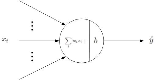
Where xi is the input, wi is the weight coefficient, and b is the offset constant. The linear output of the sensor is:

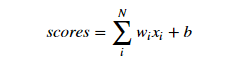
In order to simplify the calculation, we usually take b as a dimension of the weight coefficient, that is, w0. At the same time, expand the input x to a dimension of 1. In this way, the above formula is simplified as:

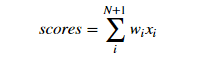
Scores is the output of the sensor. Next, judge the scores:

• If scores ≥ 0, then y_pred=1 "positive class"
• If scores < 0, then y_pred = − 1 "negative class"

Linear score calculation and threshold comparison are two processes. Finally, according to the comparison results, judge whether the sample belongs to positive or negative category.

PLA theoretical interpretation

For the binary classification problem, the perceptron model can be used to solve it. The basic principle of PLA is point by point correction. Firstly, take a classification surface at random on the hyperplane to count the points with wrong classification; Then a random error point is corrected, that is, the position of the straight line is changed to correct the error point; Then, a wrong point is randomly selected for correction, and the classification surface changes continuously until all points are completely classified correctly, and the best classification surface is obtained.

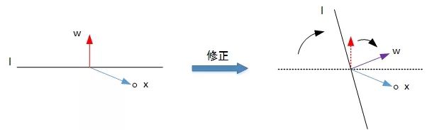
The first case is that the positive sample "y=+1" is incorrectly classified as the negative sample "y=-1". At this time, Wx < 0, that is, the included angle between w and x is greater than 90 degrees, on both sides of the classification line l. The correction method is to reduce the included angle and correct the w value so that they are on the same side of the straight line:

The schematic diagram of the correction process is as follows:

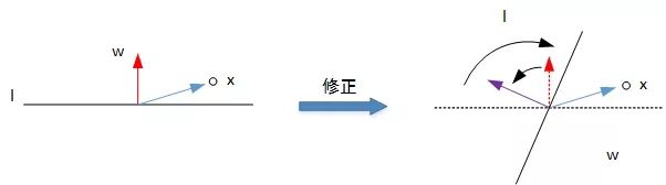
In the second case, the negative sample "y=-1" is incorrectly classified as the positive sample "y=+1". At this time, Wx > 0, that is, the included angle between w and x is less than 90 degrees, on the same side of the classification line l. The correction method is to increase the included angle and correct the w value so that they are located on both sides of the straight line:

The schematic diagram of the correction process is as follows:

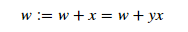
After analyzing two cases, we find that the update expression of W in PLA is the same every time: w:=w+yx. After mastering the optimization expression of each W, PLA can constantly correct all wrong classification samples and classify them correctly.

Data preparation

The data set contains 100 samples, 50 positive and 50 negative samples, and the feature dimension is 2.

import numpy as np
import pandas as pd

data = pd.read_csv('./data/data1.csv', header=None)
# Sample input, dimension (100, 2)
X = data.iloc[:,:2].values
# Sample output, dimension (100,)
y = data.iloc[:,2].values

Next, we plot the distribution of positive and negative samples on a two-dimensional plane.

import matplotlib.pyplot as plt

plt.scatter(X[:50, 0], X[:50, 1], color='blue', marker='o', label='Positive')
plt.scatter(X[50:, 0], X[50:, 1], color='red', marker='x', label='Negative')
plt.xlabel('Feature 1')
plt.ylabel('Feature 2')
plt.legend(loc = 'upper left')
plt.title('Original Data')
plt.show()

PLA algorithm

Firstly, the two features are normalized respectively, namely:

Among them, μ Is the characteristic mean, σ Is the characteristic standard deviation.

# mean value
u = np.mean(X, axis=0)
# variance
v = np.std(X, axis=0)

X = (X - u) / v

# Mapping
plt.scatter(X[:50, 0], X[:50, 1], color='blue', marker='o', label='Positive')
plt.scatter(X[50:, 0], X[50:, 1], color='red', marker='x', label='Negative')
plt.xlabel('Feature 1')
plt.ylabel('Feature 2')
plt.legend(loc = 'upper left')
plt.title('Normalization data')
plt.show()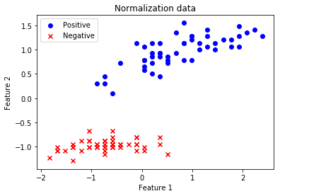

Next, initialize the prediction line, including weight w initialization:

# X plus offset
X = np.hstack((np.ones((X.shape[0],1)), X))
# Weight initialization
w = np.random.randn(3,1)

Next, calculate the scores, and compare the score function with the threshold value 0. If it is greater than zero, then y ̂ = 1, y if less than zero ̂ = −1.

s = np.dot(X, w)
y_pred = np.ones_like(y)    # Predictive output initialization
loc_n = np.where(s < 0)[0]    # Index subscript greater than zero
y_pred[loc_n] = -1

Then, select one of the samples with wrong classification and update the weight coefficient w with PLA.

# First misclassification point
t = np.where(y != y_pred)[0][0]
# Update weight w
w += y[t] * X[t, :].reshape((3,1))

Updating the weight w is an iterative process. As long as there are samples with wrong classification, it will be updated continuously until all samples are classified correctly (note that the premise is that the positive and negative samples are completely separable).

The whole iterative training process is as follows:

for i in range(100):
    s = np.dot(X, w)
    y_pred = np.ones_like(y)
    loc_n = np.where(s < 0)[0]
    y_pred[loc_n] = -1
    num_fault = len(np.where(y != y_pred)[0])
    print('The first%2d Number of points with wrong classification in the last update:%2d' % (i, num_fault))
    if num_fault == 0:
        break
    else:
        t = np.where(y != y_pred)[0][0]
        w += y[t] * X[t, :].reshape((3,1))

After the iteration, get the updated weight coefficient w and draw what the classification line looks like at this time.

# First coordinate of line (x1, y1)
x1 = -2
y1 = -1 / w[2] * (w[0] * 1 + w[1] * x1)
# Second coordinate of line (x2, y2)
x2 = 2
y2 = -1 / w[2] * (w[0] * 1 + w[1] * x2)
# Mapping
plt.scatter(X[:50, 1], X[:50, 2], color='blue', marker='o', label='Positive')
plt.scatter(X[50:, 1], X[50:, 2], color='red', marker='x', label='Negative')
plt.plot([x1,x2], [y1,y2],'r')
plt.xlabel('Feature 1')
plt.ylabel('Feature 2')
plt.legend(loc = 'upper left')
plt.show()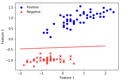

In fact, the efficiency of PLA algorithm is quite good. It only needs several updates to find a classification line that can completely classify all samples correctly. Therefore, it is concluded that for the case of linear separability of positive and negative samples, PLA can obtain the correct classification line after finite iterations.

Summary and questions

The data imported in this paper is linearly separable, and PLA can be used to obtain classification lines. However, if the data is not linearly separable, that is, no straight line can be found to completely classify all positive and negative samples correctly. In this case, it seems that PLA will update and iterate forever, but no correct classification line can be found.

How to use PLA algorithm in the case of linear indivisibility? We will improve and optimize PLA next time.